Workshop 5 + Solutions - Exploring Many Continuous Variables
- Visualising multivariate continuous data using:
pairsto produce a scatterplot matrixparallelplotpackage to produce a parallel coordinate plot
- Introduce plots useful (and potentially not so useful) for getting
an overview of a large data set
- Correlation plots as a summary of a scatterplot matrix
- Using heatmaps, glyphs, or faces to visualise and compare the cases in the data
You will need to install the following packages for today’s workshop:
latticefor theparallelplotfunction
install.packages("lattice")1 Multivariate continuous data
1.1 Scatterplots
Scatterplot matrices (sometimes inelegantly called “sploms”) are tables of scatterplots with each variable plotted against all others. They give excellent overviews of the relationships between many variables at once, and allow us to identify - by eye - any striking patterns of behavior between pairs of variables. In particular, if we’re interested in building a model for one particular variable then drawing a scatterplot matrix gives us a quick way of identifying which other variables in the data set are associated with in (and hence potentially useful predictors in a model), and which are not (and can likely be ignored).
Download data: marks
This data set (from the very end of Workshop 2) contains the exam marks of 88 students taking an exam on five different topics in mathematics. The data contain the separate marks for each topic on a scale of 0-100:
MECH- mechanicsVECT- vectorsALG- algebraANL- analysisSTAT- statistics
As the data are all numeric, we can immediately draw a scatterplot matrix which will be a 5x5 grid of plots:
pairs(marks,pch=16)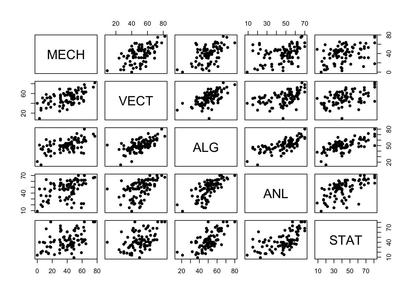
There are a number of things we can observe:
- Almost all of these variables have a positive association, though some are stronger than others. High (low) performance on one subject seems to be connected with high (low) performance on other subjects.
- The strongest association looks to be between Algebra and Analysis - two sub-disciplines of pure maths.
- Statistics and Mechanics look to have the weakest association - Statistics and Theoretical Physics are conceptually very different
- There are some very low and very high marks, including a single very
low mark on
VECT
As the relationships are reasonably linear, the correlation will give us a numerical summary of the strength of the relationships
cor(marks)## MECH VECT ALG ANL STAT
## MECH 1.0000000 0.5534052 0.5467511 0.4093920 0.3890993
## VECT 0.5534052 1.0000000 0.6096447 0.4850813 0.4364487
## ALG 0.5467511 0.6096447 1.0000000 0.7108059 0.6647357
## ANL 0.4093920 0.4850813 0.7108059 1.0000000 0.6071743
## STAT 0.3890993 0.4364487 0.6647357 0.6071743 1.0000000Let’s use colour to identify this low mark (and possible outlier) to see where it falls within the distribution of the other marks:
library(scales)
colours <- rep('black',length=nrow(marks)) ## create a vector of same length as the data, by repeating "black"
colours <- alpha(colours,0.4) ## use some transparency to fade most of the cases
which(marks$VECT<10)     ##  find out which row in the data set has a VECT mark below 10
## [1] 81colours[which(marks$VECT<10)] <- 'red' ## replace the colour for that row with "red"
pairs(marks,col=colours,pch=16) ## now draw the plot using our custom colours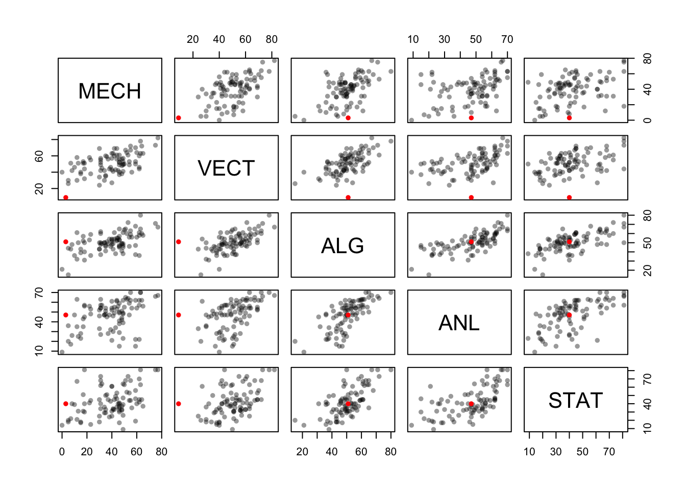
We find that this student did reasonably well on the other exams, but really didn’t do well with Mechanics or Vectors! These two topics are quite closely related, so this seems quite a natural outcome.
1.2 Parallel coordinate plot
We can also try a parallel coordinate plot (PCP). Parallel coordinates can be quite effective for showing multiple variables, and among the most common subjects of academic papers in visualization. While initially confusing, they are a very powerful tool for understanding multi-dimensional numerical datasets. To understand how the plot is produced, let’s look at a portion of the data:
| MECH | VECT | ALG | ANL | STAT |
|---|---|---|---|---|
| 77 | 82 | 67 | 67 | 81 |
| 63 | 78 | 80 | 70 | 81 |
| 75 | 73 | 71 | 66 | 81 |
| 55 | 72 | 63 | 70 | 68 |
| 63 | 63 | 65 | 70 | 63 |
| 53 | 61 | 72 | 64 | 73 |
Imagine each of these columns being mapped onto a vertical axis. Each
data value would end up somewhere along the line, scaled to lie between
the minimum at the bottom and the maximum at the top. A pure collection
of points would not be terribly useful, however, so the points belonging
to the same data point (row) are connected with lines. Drawing the plot
for these few observations gives us:
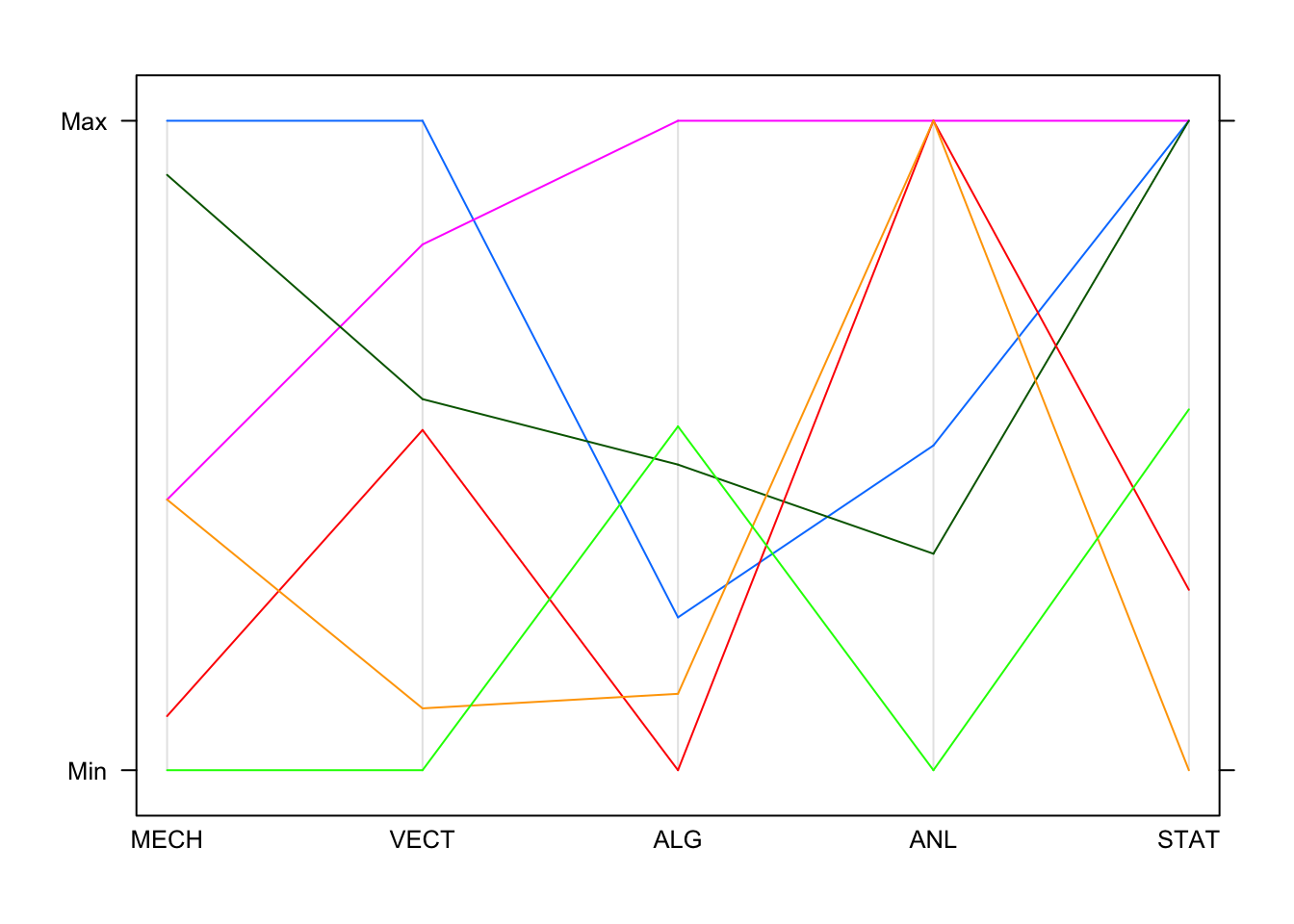
By default, each line is drawn in a different colour. This is fine
for a small number of cases, but becomes messy with a lot of data - in
this case it is best to override the colouring. You can also make the
lines fatter by increasing the line width, e.g. add the
lwd=2 argument to the plot command.
Now, if we draw all of the data we create the characteristic jumble of lines parallel coordinates are famous for. Colouring in the same was as we did the scatterplot, we get this:
library(lattice)
parallelplot(marks,horizontal=FALSE,col=colours)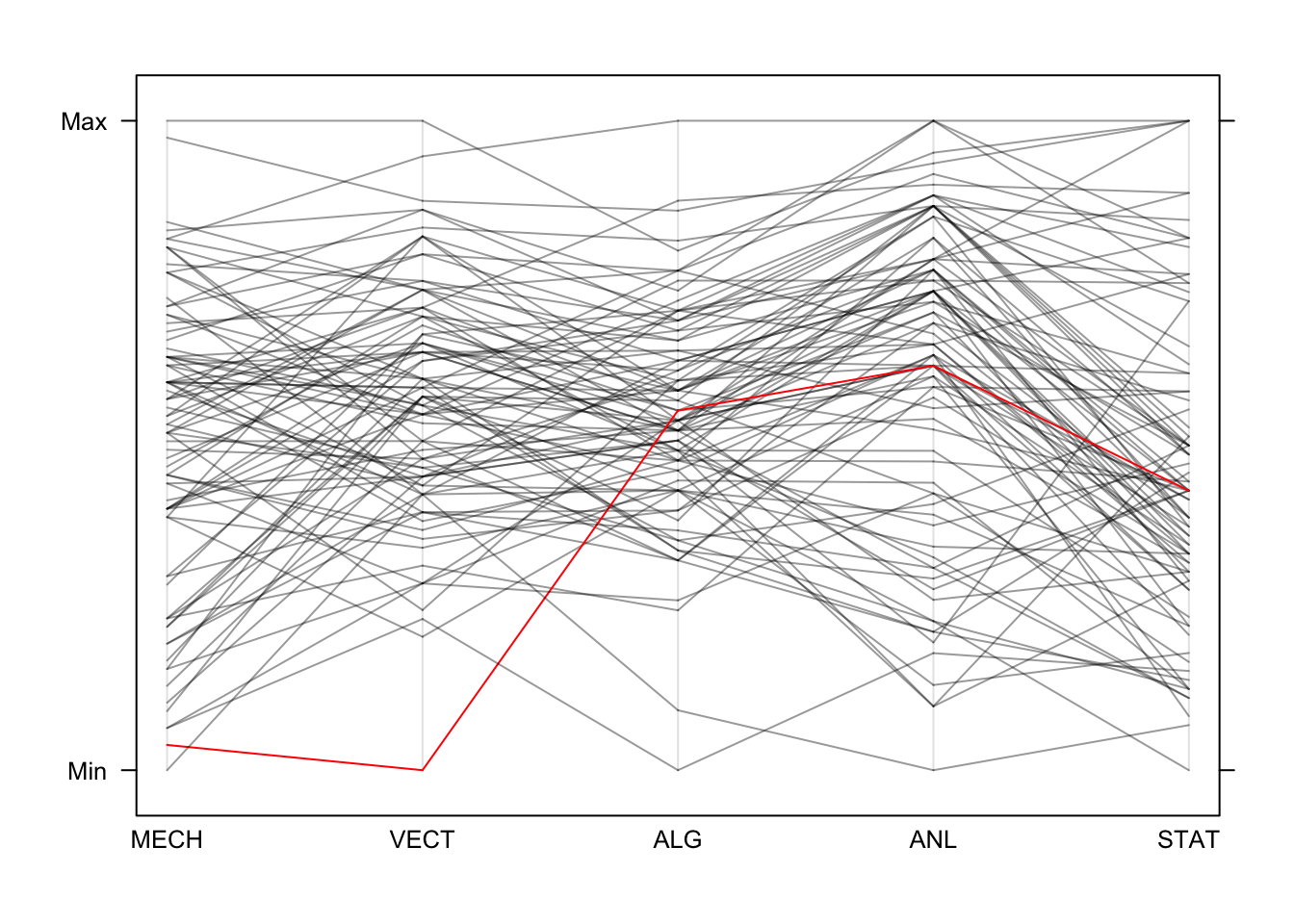
We can easily trace the red line’s performance across the different
exams. When there are bigger groups defined in the data, we can get the
parallelplot function to colour the groups automatically by
passing the grouping variable into the groups argument.
Unfortunately, we don’t have a group variable here but we can make one
to illustrate the technique. We could have equally created a group
variable to identify and highlight our outlier above.
## make a categorical variable to separate high scores on STATistics
hiStat <- factor(marks$STAT<70)
parallelplot(marks,horizontal=FALSE,groups=hiStat)
So high achievers on Stats generally do well on Analysis. Some do
well on the other subjects, but performance drops and becomes more
variable as we move left in the plot! One feature we can read from the
PCP is when the values correspond to the same data point - for example,
we can see the top student on algebra (ALG) was also top on
analysis (ANL) and stats (STAT), and did
pretty well on mechanics (MECH).
In the scatterplot matrix, since each panel only displays two variables it is not always clear how the points in each panel relate to the points in the other panels.
1.3 Data set 1: Crime in the USA
Download data: crime.us
The data set crime.us includes the crime totals and
rates (per 100,000 population) for 50 US states during 2009. There are
16 variables, which we can separate into a small number of groups:
StateandPopulation- the name and population of the state- Totals: total crime numbers for 7 crime categories -
Murder,Rape,Robbery,Assault,Burglary,LarcenyTheft,MotorVehicleTheft - Rates: rates per 100,000 for 9 crime categories -
ViolentCrimeRate,MurderRate,RapeRate,RobberyRate,AssaultRate,BurglaryRate,LarcenyTheftRate,MotorVehicleTheftRate
- First, take a quick look at the first few rows of the data using the
headfunction. - As the data are a mix of continuous and categorical variables, we
can’t simply pass the whole data set into the
pairsfunction. - Use the
namesfunction to get a list of the variable names. Which columns correspond to the rates for the various crimes? - Draw a scatterplot matrix of just the 9 crime rates. Hint: select a subset of the columns corresponding to the variables of interest.
- What patterns and associations can you see?
- The crimes can be divided into Violent crimes (Murder, Rape, Robbery, Assault), and Property crimes (Burglary, Larceny Theft, Motor Vehicle Theft). Do you find different patterns of association among similar crimes?
- Are there any obvious outliers? If so, try and identify which State they are from the data, and use colour to highlight them on your scatterplot.
- Make a parallel coordinate plot and use it to investigate these outliers across all the variables.
- Have a quick look at the scatterplot matrix of the crime totals. Why do you think we focussed on the rates in our analysis above?
head(crime.us)## State Population Murder Rape Robbery Assault Burglary LarcenyTheft MotorVehicleTheft MurderRate
## 1 Alabama 4708708 323 1504 6259 13093 48837 117711 11081 6.9
## 2 Alaska 698473 22 512 655 3232 3597 15291 1689 3.1
## 3 Arizona 6595778 354 2110 8099 16366 53412 155184 25986 5.4
## 4 Arkansas 2889450 179 1368 2582 10830 34764 68171 6103 6.2
## 5 California 36961664 1972 8713 64093 99681 230137 615456 164021 5.3
## 6 Colorado 5024748 175 2242 3387 11172 26649 94861 12458 3.5
## RapeRate RobberyRate AssaultRate BurglaryRate LarcenyTheftRate MotorVehicleTheftRate
## 1 31.9 132.9 278.1 1037.2 2499.9 235.3
## 2 73.3 93.8 462.7 515.0 2189.2 241.8
## 3 32.0 122.8 248.1 809.8 2352.8 394.0
## 4 47.3 89.4 374.8 1203.1 2359.3 211.2
## 5 23.6 173.4 269.7 622.6 1665.1 443.8
## 6 44.6 67.4 222.3 530.4 1887.9 247.9names(crime.us)## [1] "State" "Population" "Murder" "Rape"
## [5] "Robbery" "Assault" "Burglary" "LarcenyTheft"
## [9] "MotorVehicleTheft" "MurderRate" "RapeRate" "RobberyRate"
## [13] "AssaultRate" "BurglaryRate" "LarcenyTheftRate" "MotorVehicleTheftRate"## rates are columns 10 to 16rates <- crime.us[,10:16]
pairs(rates)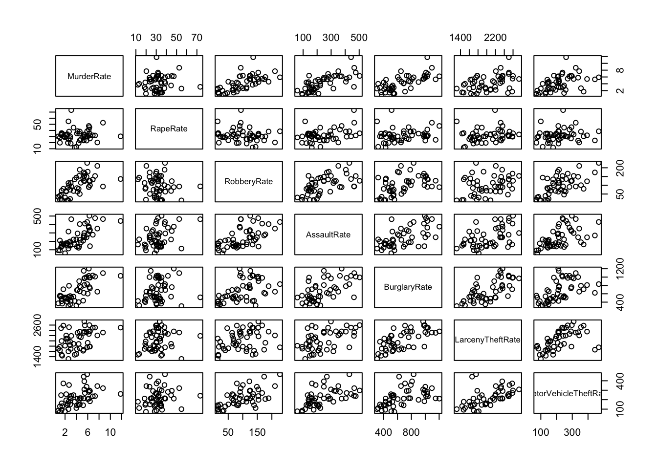
## some obvious associations here. Most crime rates seem to have a positive association (i.e. higher Robbery rates are associated with higher Assault Rates, etc)
## The rate for Rape however does not appear associated, suggesting this is somehow a different "type" of crime not clearly associated with other criminal behaviours
## The crimes within the suggested Violent/Property groups generally seem more strongly associated to each other than to those from the other group of crimes (excl. Rape for reasons above)
## There are some points with unusually high values, namely on Murder, Rape and MotorVehicleTheft
# Murder
crime.us[crime.us$MurderRate>11,]$State## [1] "Louisiana"# Rape
crime.us[crime.us$RapeRate>70,]$State## [1] "Alaska"#
crime.us[crime.us$MotorVehicleTheftRate>440,]$State## [1] "California" "Nevada"## how to highlight? test the states to see if they match one of the ones we found
hilight <- crime.us$State %in% c("Louisiana","Alaska","California","Nevada")
pairs(rates,pch=16,col=ifelse(hilight,'red','black'))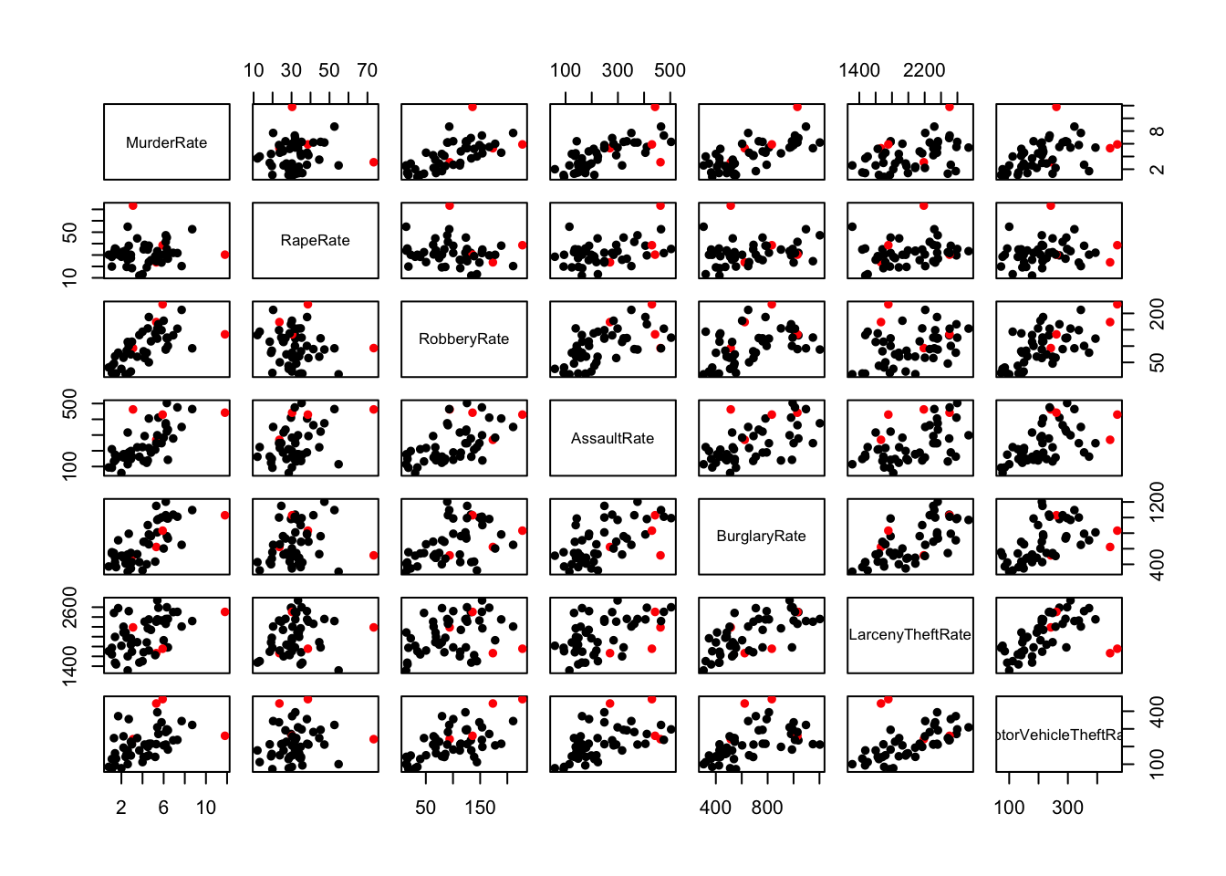
## some of the 'extremes' are not extremes on all the varaibles, need to investigate more closelyparallelplot(crime.us[,10:16],horizontal=FALSE,col=ifelse(hilight,'red','black'))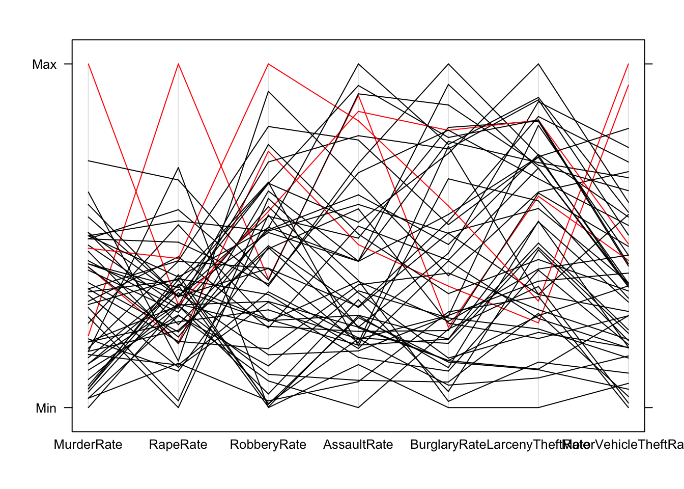
## it appears that the states are usually only extreme on one of the variables and relatively ordinary on the others
## to look at this in more detail, we should single out the states, for example
parallelplot(crime.us[,10:16],horizontal=FALSE,col=ifelse(crime.us$State=="Louisiana",'red','black'))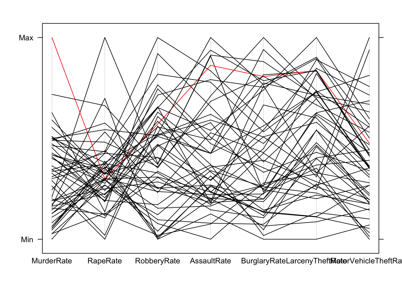
pairs(crime.us[,10:16],pch=16,col=ifelse(crime.us$State=="Louisiana",'red','black'))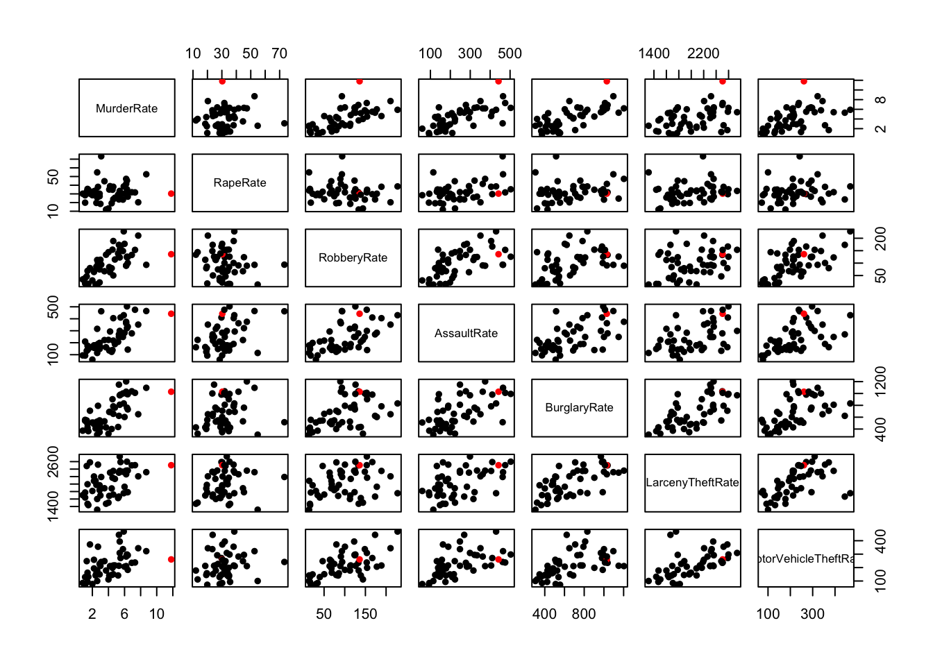
## shows Louisiana as extreme on Murder, and high -but not surprisingly so- on the otherspairs(crime.us[,3:9])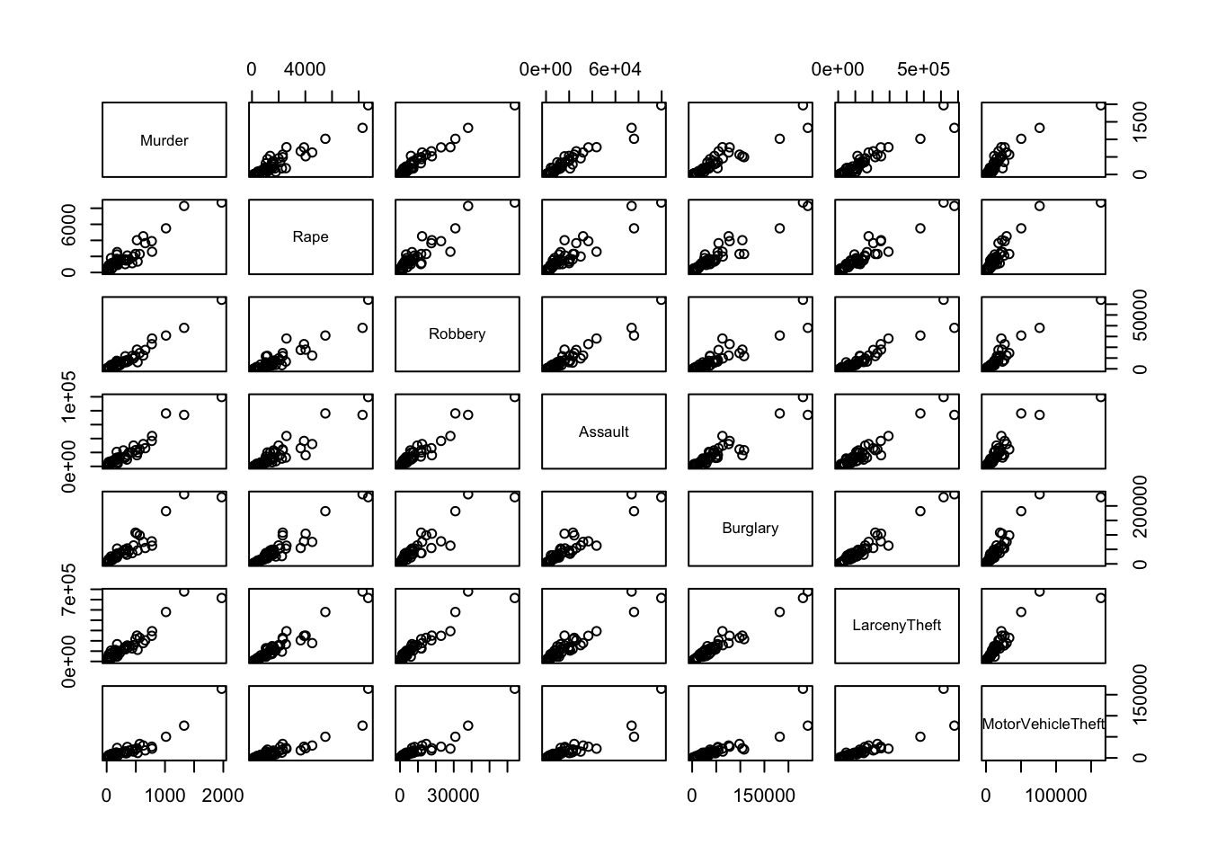
## the counts are on very different scales depending on the state. Understandable, since each state has different sizes of populations, and hence would expect different *numbers* of crimes.
## Looking at the rates removes the influence of state size on the analysis allowing us to make comparisons more easily.
1.4 Data set 2: Crabs
Download data: crabs
The crabs data concerns different measurements made on
50 crabs each of two colours and both sexes of the species Leptograpsus
variegatus, collected in Australia. This gives 200 total data points
on each of the following variables:
sp- the colour species of crab, either"B"for blue or"O"for orangesexindex- index 1:50 within each groupsFL- frontal lobe size (mm)RW- rear width (mm)CL- carapace length (mm)CW- carapace width (mm)BD- body depth (mm).
- Again, take a quick look at the first few rows of the data using the
headfunction. - Make a quick scatterplot matrix of the five measurement variables. What do you see?
- Try a parallel coordinate plot, how does the strong association appear in the plot?
head(crabs)## sp sex index FL RW CL CW BD
## 1 B M 1 8.1 6.7 16.1 19.0 7.0
## 2 B M 2 8.8 7.7 18.1 20.8 7.4
## 3 B M 3 9.2 7.8 19.0 22.4 7.7
## 4 B M 4 9.6 7.9 20.1 23.1 8.2
## 5 B M 5 9.8 8.0 20.3 23.0 8.2
## 6 B M 6 10.8 9.0 23.0 26.5 9.8pairs(crabs[,4:8])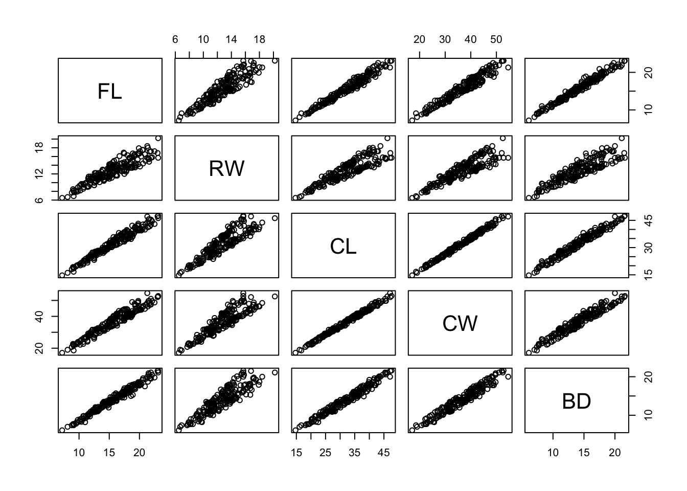
## incredibly strong correlations! There's a strong linear relationship here - this is quite common for biological measurements of living things. Big crabs/people/giraffes will have large limbs/heads/torsos/etc.
## Note that in the RW column/row of plots there almost appears to be two different straight-line relationships. Is this an effect related to one of the categorical variables?
parallelplot(crabs[,4:8],horizontal=FALSE)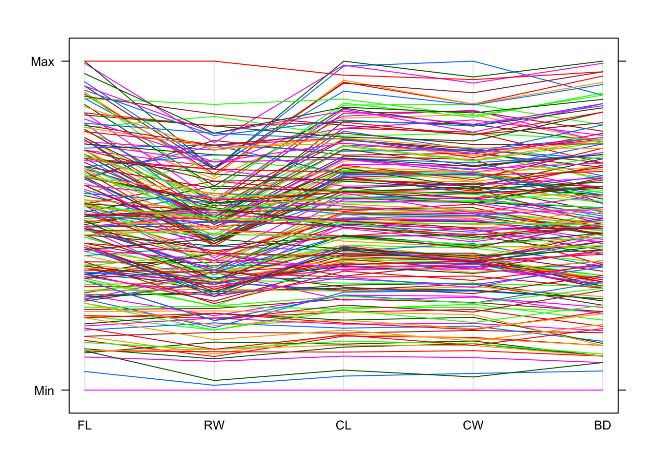
## arguably this is harder to read, and certainly less striking!
## however, we can see that all the lines are comparatively straight and don't jump up and down as much as the previous example. In other words, if the data is big on one variable then that data point is generally big on the others too, which is the essence of a positive association.groups argument to a categorical variable which
defines the groups.
- Redraw your parallel coordinate plot, but add the extra argument
groups=crabs$sp. - Can you figure out which colour is which species? Hint
identify the colour of the smallest
FLvalue, then find that in the data. - What differences can you see between the different species?
- Now colour by
sexinstead - do you find any featuers of interest?
parallelplot(crabs[,4:8],horizontal=FALSE,groups=crabs$sp)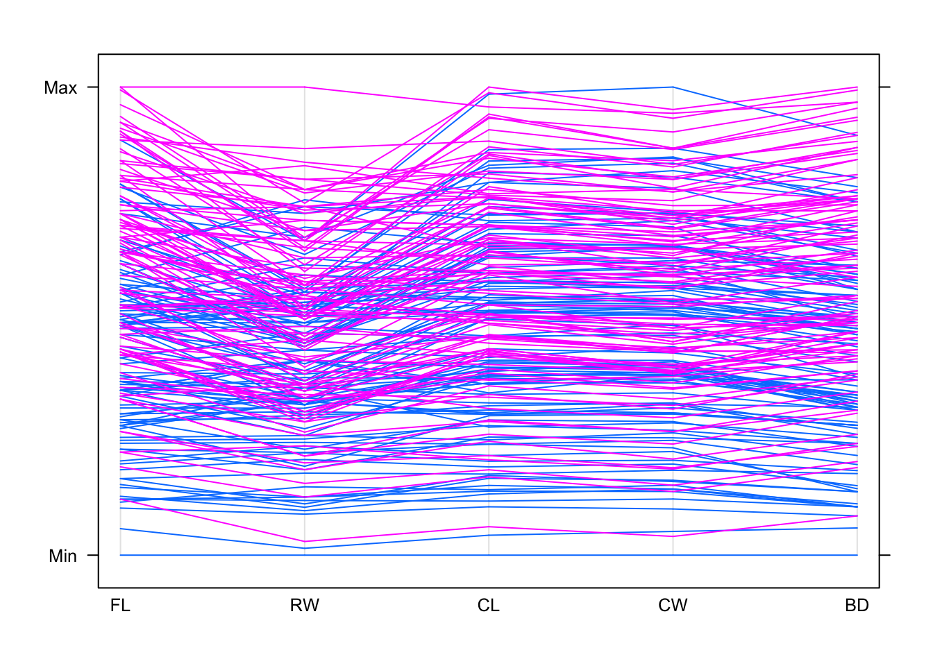
## now coloured by species, which is one of "B" or "O"
## The smallest value on FL is coloured blue - so what species is that?
crabs[which.min(crabs$FL),]
## sp sex index FL RW CL CW BD
## 51 B F 1 7.2 6.5 14.7 17.1 6.1## So this is a "B" species crab
## In general, the blue lines are lower down the plot and the pink are higher up - so "B" crabs appear to be generally smallerparallelplot(crabs[,4:8],horizontal=FALSE,groups=crabs$sex)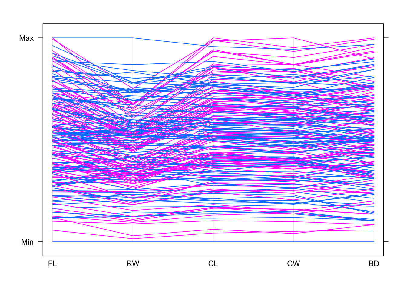
## the sex effect is much less clear, with no clear differentiation between the groups.
## in particular both the largest and smallest on FL and RW are both the same sex
One problem with data like these is that the many strong associations
mean that large values on one variable are associated with other large
values, since it is the overall size of the animal that changes most and
all the features remain in roughly the same proportion. To highlight any
deviations from the usual pattern, we could look at the relative sizes
of the different features - in this case compared to the carapace length
(CL).
## divide `FL` by `CL` and create a new variable in the data frame called `FLCL`
crabs$FLCL <- crabs$FL/crabs$CL
## repeat!
crabs$RWCL <- crabs$RW/crabs$CL
crabs$CWCL <- crabs$CW/crabs$CL
crabs$BDCL <- crabs$BD/crabs$CL
Of course, now we only have four variables to work with (since
CL/CL just gives us 1, so that’s not useful).
- Scale the variables using the code above, and make a new plot of these four new variables and colour by species.
- Can you spot any interesting differences now?
- Experiment with plotting the variables in a different order to emphasise the differences between the two groups.
- If you had to classify the crabs into two species, which variables would you use and how would you classify?
parallelplot(crabs[,c(9:12)],groups=crabs$sp,horizontal=FALSE)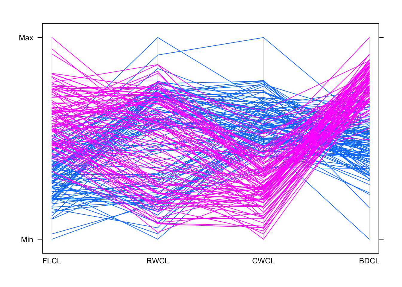
## This shows some dramatic differences now
## "B" species (blue) have lower values of FLCL and higher SWCL and BDCL, with the other species doing largely the opposite
## RWCL doesn't look helpful for separating the groups
## try a different variable order...
parallelplot(crabs[,c(10,11,9,12)],groups=crabs$sp,horizontal=FALSE)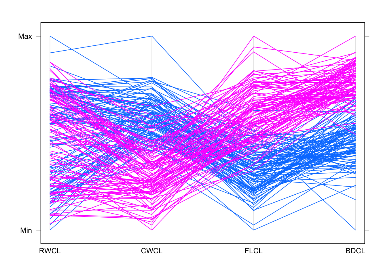
1.5 Variations on Standard Plots : Radar charts
If you thought the parallel coordinate plot was too much, then the radar chart (also called spider or web or polar charts) will be a step too far. While similar in concept to the parallel coordinate plot, the radar chart arranges each variable’s axis as equally-spaced spokes around a circle. The data points are still drawn with lines on these radial axes, but now their connnecting lines wind around the centre point.
library(fmsb)
colours <- alpha(rep('black',length=nrow(marks)),0.4)
colours[81] <- 'red'
radarchart(marks,maxmin=FALSE, pcol=colours, plty=1)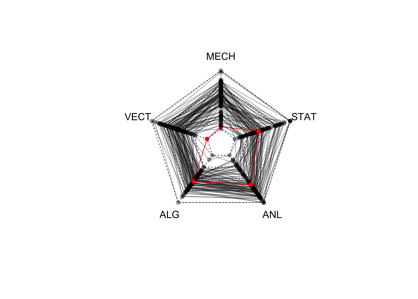
2 Getting an Overview
When you first start work on a dataset it is important to learn what variables it includes and what the data are like. There will usually be some initial analysis goals, but it is still necessary to look over the dataset to ensure that you know what you are dealing with. There could be issues of data quality, perhaps missing values or outliers, and there could be some surprising basic statistics.
There are many ways to get an initial impression of a new data set, and we’ve seen a lot of the techniques already:
- Inspect the data values - use the
headorViewfunctions - Calculate simple statistical summaries - use the
summaryorfivenumfunctions - Separate the quantitative from categorical variable - use subsetting to split the data up
- Draw simple univariate summary plots for each variable -
use
par(mfrow=c(x,y))to create a grid of plots, and usehistorbarplotto plot the individual variables; useboxplotto draw a boxplot of all quantitative variables. - Look for associations and relationships - use the
pairsfunction to draw a scatterplot matrix of the quantitative variables, or a matrix of two-way mosaic plots of the categorical variables.
A correlation plot or corrplot can help give a summary version of a scatterplot matrix, useful when the number of variables to plot is large.
In addition to these techniques, there are a few plot types that can help us visualise the entire data set in one go. Rather than focussing on general behaviour between variables, these methods focus on visualising the different data points to see how the points differ from one another. We’ll look at three graphs, suitable for getting an overview of quantitative variables:
- Corrplots
- A heatmap
- A glyph or star plot
- Chernoff faces
To illustrate these plots, we’ll use the US crime statitsics data set from Workshop 3.
Download data: crime.us
2.1 Corrplots
A simple summary of the strength of the (linear) association between
a pair of variables is its correlation. When we have a collection of
quantitative variables, we can evaluate the correlation matrix using the
cor function. Values close to \(1\) or \(-1\) indicate strong linear relationships,
values close to \(0\) indicate a lack
of a linear relationship.
The correlation matrix can be visualised as a simple alternative to a scatterplot matrix suitable for problems when the number of variables is too large to read the individual scatterplots.
round(cor(crime.us[,10:16]),2)## MurderRate RapeRate RobberyRate AssaultRate BurglaryRate LarcenyTheftRate
## MurderRate 1.00 0.07 0.66 0.71 0.72 0.42
## RapeRate 0.07 1.00 -0.16 0.38 0.20 0.18
## RobberyRate 0.66 -0.16 1.00 0.58 0.49 0.32
## AssaultRate 0.71 0.38 0.58 1.00 0.61 0.50
## BurglaryRate 0.72 0.20 0.49 0.61 1.00 0.69
## LarcenyTheftRate 0.42 0.18 0.32 0.50 0.69 1.00
## MotorVehicleTheftRate 0.49 0.15 0.63 0.54 0.52 0.53
## MotorVehicleTheftRate
## MurderRate 0.49
## RapeRate 0.15
## RobberyRate 0.63
## AssaultRate 0.54
## BurglaryRate 0.52
## LarcenyTheftRate 0.53
## MotorVehicleTheftRate 1.00library(corrplot)
corrplot(cor(crime.us[,10:16]),tl.cex=0.75)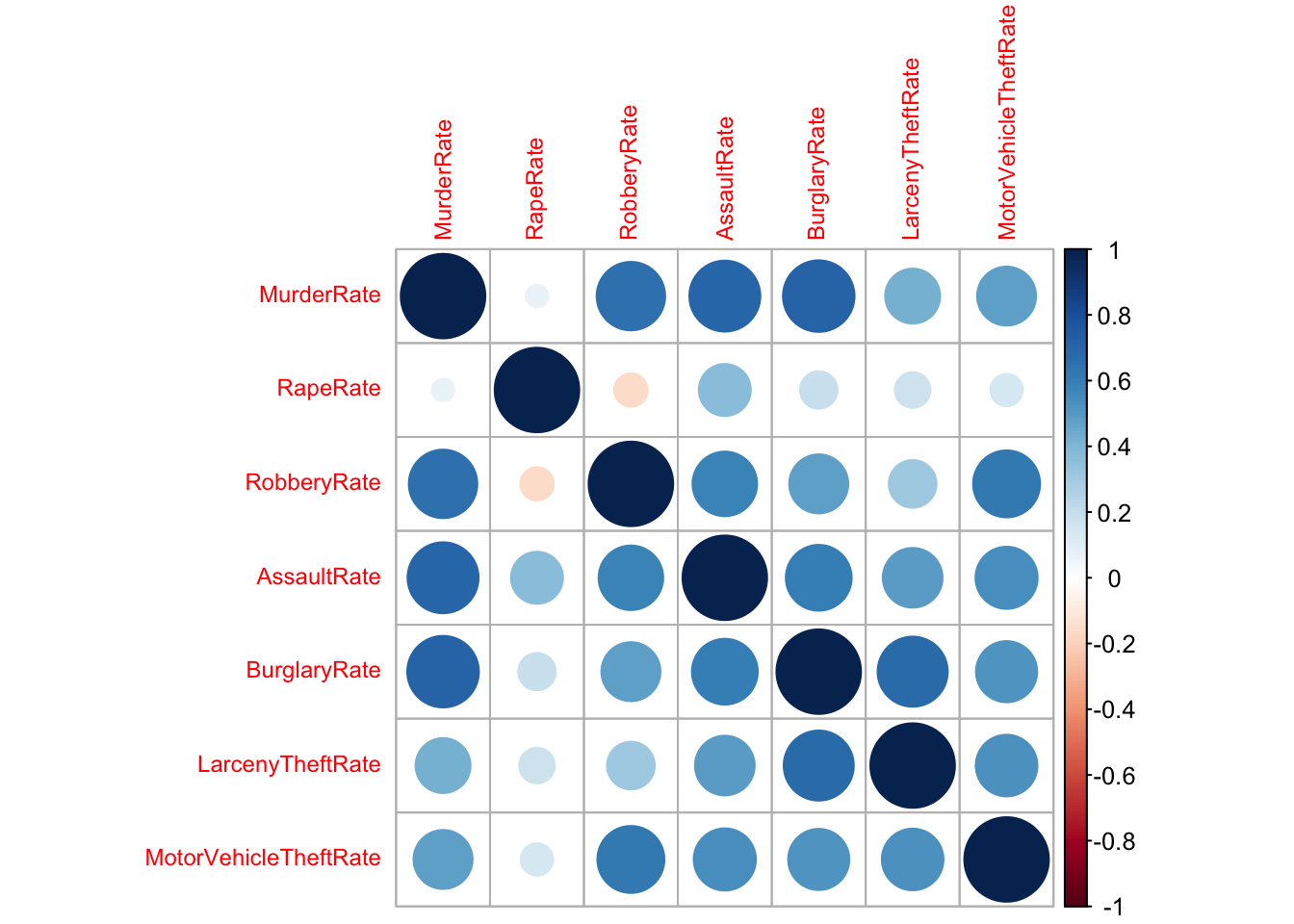
2.2 Heatmaps
With a heatmap each data point is represented by a row and each variable by a column. The individual cells are coloured according to the case value relative to the other values in the column. For this purpose, the variables are standardised individually, either with a normal transformation to \(z\) scores (i.e. subtract the mean and divide by the standard deviation) or adjusted to a scale from minimum to maximum.
We will use the function heatmap.2 from the
gplots package, which uses a \(z\) scaling of the data. Let’s draw a
heatmap of the crime rate variables (columns 10 to 16)
## add the state names as row labels
rownames(crime.us) <- crime.us$State
## draw the heatmap
library(gplots)
hmap <- heatmap.2(as.matrix(crime.us[,10:16]),
                  scale='column', # scale the data by the column
                  trace='none', cexCol=0.75) # shrink the column labels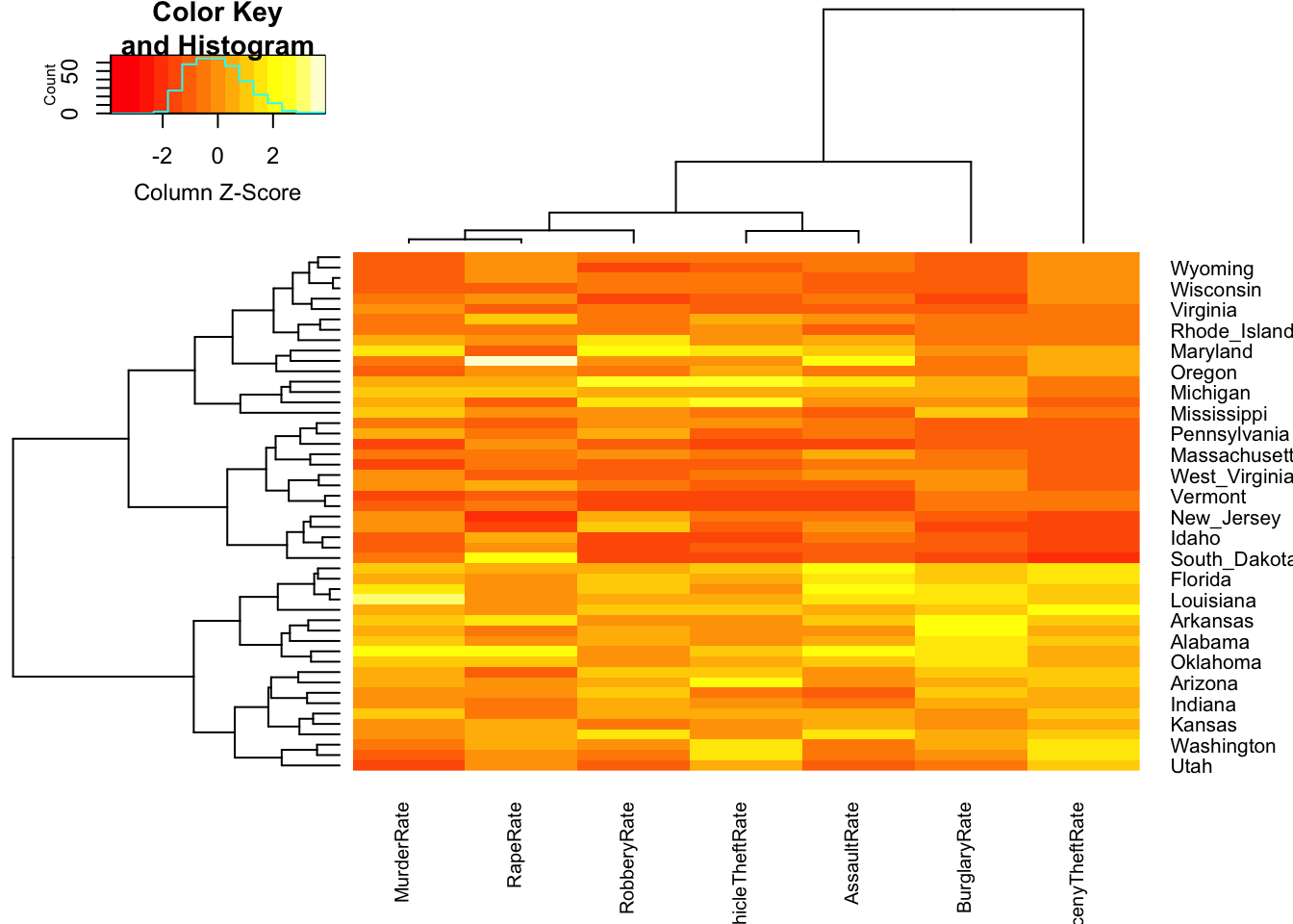
The colours within each column range from red (low values) through to
yellow (high values). The rows in the data have been permuted to
emphasise difference between the different cases, and here we can
observe a block of data points in the lower half of the plot with
particularly large values (lots of yellows) of Larceny and Burglary.
Looking closer at the labels, we note that most of the states in this
group seem to correspond to States in the South. We can also spot a
white cell in the RapeRate column corresponding to Alaska,
which we previously noted.
The tree structures on the left and above the plot show a clustering of the data cases (left) into groups of similar points, and a clustering of the variables (above). You’ll see more on clustering later.
2.3 Glyphs
With glyphs, each case is represented by a multivariate symbol reflecting the case’s variable values. As for heatmaps, each variable must be standardised in some way first and this can influence the w
stars(crime.us[,10:16],draw.segments=TRUE)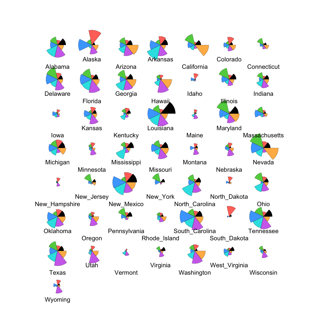
We can modify this to show the data cases in the same order as the
heatmap by extracting the ordering from the heatmap output (in the
rowInd component) and using it to rearrange our data set.
We can also set custom colours to make things prettier!
stars(crime.us[hmap$rowInd,10:16], draw.segments=TRUE)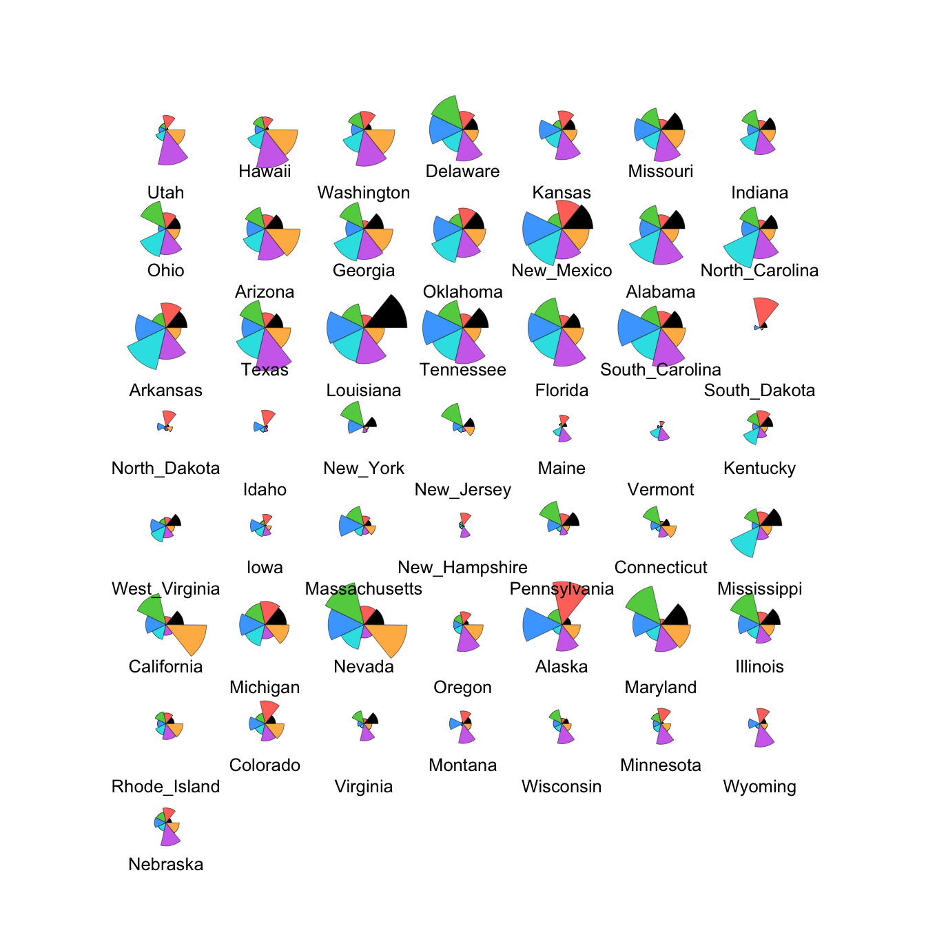
The large values on the southern states stand out quite clearly now in the top block of cases.
2.4 Chernoff faces
This one is a little nuts, and is more of a curiosity than anything.
Chernoff faces display multivariate data in the shape of a human face. The idea behind using faces is that humans easily recognize faces and notice small changes without difficulty. Chernoff faces handle each variable differently. Because the features of the faces vary in perceived importance, the way in which variables are mapped to the features should be carefully chosen.
library(TeachingDemos)
faces(crime.us[hmap$rowInd,10:16])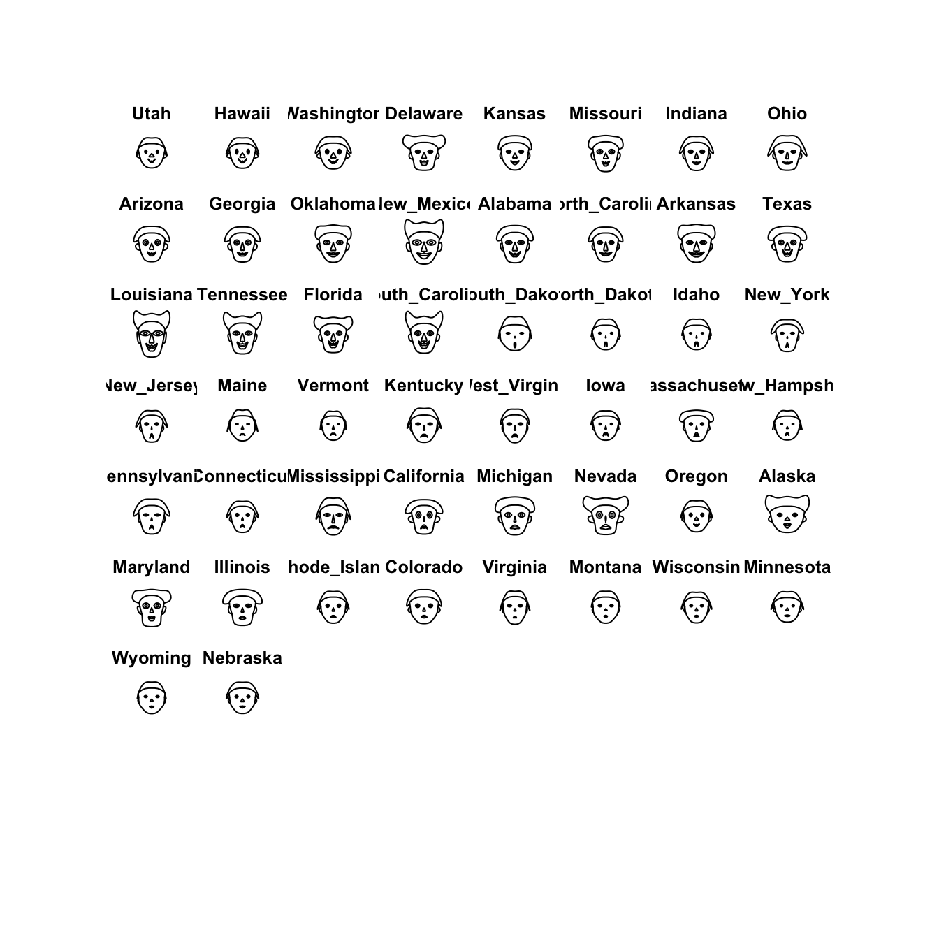
I’m not sure its particularly helpful or particularly effective as a visualisation, but it is another variation on the idea of a glyph plot.
2.5 Data Set: The Guardian University League Table 2013
Download data: uniranks
We’ve looked at these data before, in Lecture 2 where we explored the parallel coordinate plot. Let’s use this as an example data set for exploring some of the techniques above. The data set contains a number of variables for 120 UK universities:
Rank- Overall rank of the University in the League TableInstitution- University nameUniGroup- Universities can be a member of one of five groups, 1994 Group, Guild HE, Million+, Russell, University Alliance, or noneHesaCode- University’s Higher Education Statistics Agency ID codeAvTeachScore- Average Teaching ScoreNSSTeaching- University’s National Student Survey teaching scoreNSSOverall- University’s NSS overall scoreSpendPerStudent- University expenditure per student (depends on subject)StudentStaffRatio- Student to Staff ratioCareerProspects- Proportion of graduates in appropriate level employment or full-time study within six months of graduationValueAddScore- ”Based upon a sophisticated indexing methodology that tracks students from enrolment to graduation, qualifications upon entry are compared with the award that a student receives at the end of their studies.” (Guardian)EntryTariff- Value dependent on the average points needed to get on the university’s coursesNSSFeedback- University’s NSS feedback score
- Load the data, and extract the numerical data variables.
- Apply the graphical techniques above - what features can you see?
- How would you explore behaviour of the different University groups?
uni <- uniranks[,-c(1:4)]
uni <- uni[,c(3,1:2,4:9)] ## put the overall score column first
corrplot(cor(uni))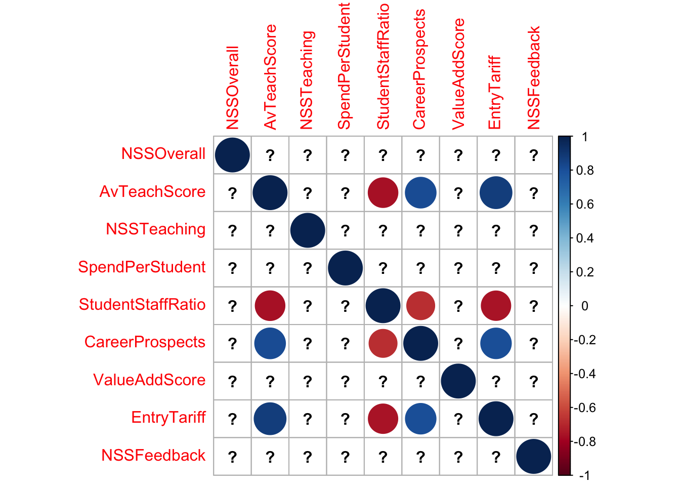
## some strong correlations here.
## a lot of '?'s - these indicate missing values
hmap <- heatmap.2(as.matrix(uni),
scale='column', # scale the data by the column
trace='none', cexCol=0.75) # shrink the column labels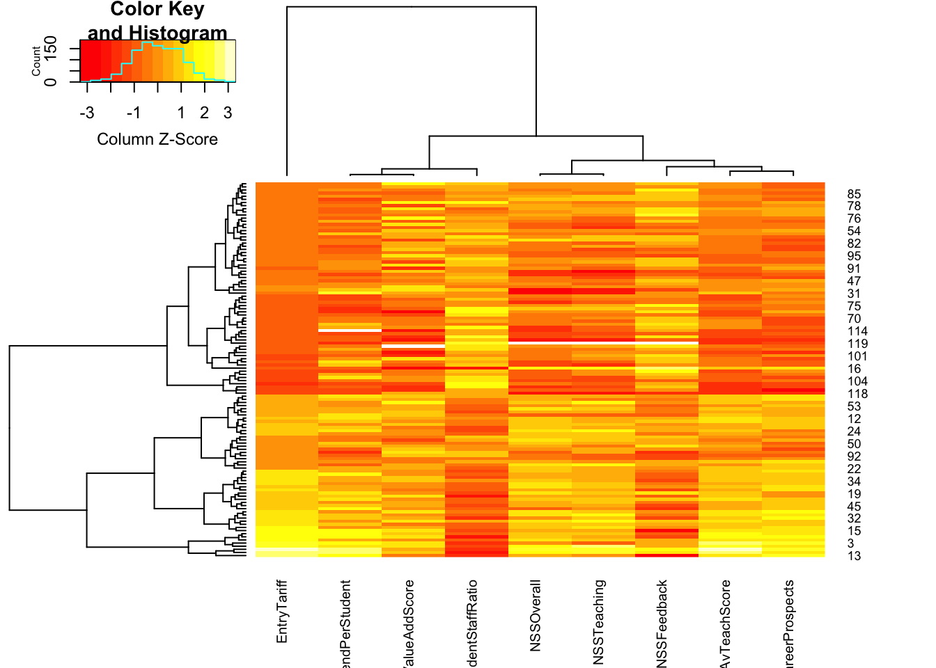
## here we can perhaps most easiliy see the same correlation patterns - e.g. the last two columns typically take similarly high/low values, suggesting a positive correlation. The studentStaffRatio behaves in the opposite direction, with lower student staff ratios corresponding to higher scores elsewhere.stars(uni, draw.segments=TRUE)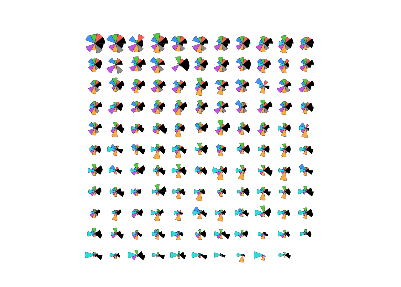
## the universities are in descending rank order, so we can see the scores shrinking as we move from top to bottom and go down the ranking.3 More Practice
3.1 Data set: Fertility in Switzerland
The built-in R dataset swiss contains a standardised
fertility measure and various socio-economic indicators for each of the
47 French-speaking provinces of Switzerland in about 1888. The six
variables it contains are:
- Fertility - ‘common standardized fertility measure’
- Agriculture - % of males involved in agriculture as occupation
- Examination - % draftees receiving highest mark on army examination
- Education - % education beyond primary school for draftees.
- Catholic - % ‘catholic’ (as opposed to ‘protestant’).
- Infant.Mortality - live births who live less than 1 year.
- Draw a parallel coordinate plot of all six variables
- Are there any cases that might be outliers on one or more variables?
- What can you say about the distribution of the variable
Catholic? - Construct a new variable with values
Highfor all provinces with more than 80% Catholics andLowerfor the rest. Draw a pcp coloured by the groups of the new variable. How would you describe the features you see?
3.2 Data set: Bodyfat
Download data: bodyfat
The dataset bodyfat gives estimates of the percentage of
body fat (bodyfat) of 252 men, determined by underwater
weighing, alog with 10 body circumference measurements, height, weight
and body density. The data set has often been used to illustrate
regression to see if body fat percentage can be predicted from the other
variables.
- Draw a parallel coordinate plot and attempt to answer the following
questions (don’t look at other plots just yet)
- Are there any outliers? What can you say about them?
- Can you deduce anything about the height variable?
- What can you say about the relationship between the first two
variables
densityandbodyfat? - Do you think that the orderings of the variables is sensible? Experiment reordering the variables to try and make a more informative plot.
- Now look at the scatterplot matrix for these data.
- You may need to use transparency here!
- How would you answer the questions above using the scatterplot matrix?