Workshop 4: Factor Analysis
Workshop 4: Factor Analysis
Factor analysis (FA) is a dimension reduction technique that presents some similarities with PCA, but also marked differences. The most important distinction is that FA not only reduces the dimension, but is also a tool for latent variable modelling: FA explicitly specifies a model relating the observed variables to a smaller set of underlying unobservable factors while PCA is a data transformation tool. As a result, Factor Analysis is more powerful, but also more challenging.
Here we explore how to perform FA using R, how to read
and visualize the output, as well as good practices and pitfalls to
avoid. For a more theoretical viewpoint on FA, you are referred to the
lecture notes.
In R, FA can be performed using either fa() or
factanal().
Quality of life data
We will start by testing the factanal() function on the
quality of life data provided by WHO. You can download the data set
lifexpect.csv from Learn Ultra.
We begin by reading the data into R and analyze its
structure.
# setwd("~/Dropbox/Maths/Teaching/2024 (Epiphany) -- MATH42515 -- Data Exploration, Visualization, and Unsupervised Learning")
# file <- file.path("Datasets", "lifexpect.csv")
dat <- read.csv("lifexpect.csv")
str(dat)
## 'data.frame': 1863 obs. of 13 variables:
## $ Country : chr "Afghanistan" "Afghanistan" "Afghanistan" "Afghanistan" ...
## $ Year : int 2014 2013 2012 2011 2010 2009 2008 2007 2006 2005 ...
## $ Life.expectancy : num 59.9 59.9 59.5 59.2 58.8 58.6 58.1 57.5 57.3 57.3 ...
## $ Adult.Mortality : int 271 268 272 275 279 281 287 295 295 291 ...
## $ infant.deaths : int 64 66 69 71 74 77 80 82 84 85 ...
## $ under.five.deaths : int 86 89 93 97 102 106 110 113 116 118 ...
## $ Alcohol : num 0.01 0.01 0.01 0.01 0.01 0.01 0.03 0.02 0.03 0.02 ...
## $ healthcare.expenditure: num 73.5 73.2 78.2 7.1 79.7 ...
## $ Hepatitis.B : int 62 64 67 68 66 63 64 63 64 66 ...
## $ Polio : int 58 62 67 68 66 63 64 63 58 58 ...
## $ Diphtheria : int 62 64 67 68 66 63 64 63 58 58 ...
## $ GDP : num 612.7 631.7 670 63.5 553.3 ...
## $ Schooling : num 10 9.9 9.8 9.5 9.2 8.9 8.7 8.4 8.1 7.9 ...The data contains measurement for multiple countries and multiple years of variables that are indicators of basic quality of life. We would like to understand, through FA, if unobservable features can be extracted from this setting. The factanal() command requires a specification of the number of factors. For the moment, to keep it simple, we choose 2 factors and select only the last 5 variables.
life.fa <- factanal(dat[,-(1:8)], factors = 2)
life.fa
##
## Call:
## factanal(x = dat[, -(1:8)], factors = 2)
##
## Uniquenesses:
## Hepatitis.B Polio Diphtheria GDP Schooling
## 0.527 0.494 0.251 0.702 0.405
##
## Loadings:
##             Factor1 Factor2
## Hepatitis.B 0.684
## Polio       0.667   0.248
## Diphtheria  0.847   0.177
## GDP                 0.541
## Schooling   0.230   0.736
##
##                Factor1 Factor2
## SS loadings      1.689   0.932
## Proportion Var   0.338   0.186
## Cumulative Var   0.338   0.524
##
## Test of the hypothesis that 2 factors are sufficient.
## The chi square statistic is 1.22 on 1 degree of freedom.
## The p-value is 0.27What do we observe?
Recall from lectures, that FA decomposes the estimated covariance matrix as \[ \Sigma_X = LL^\top + \Sigma_{\epsilon} \]
Uniquenesses
The uniquenesses range from 0 to 1. These are the diagonal entries of the matrix \(\Sigma_{\epsilon}\). They are the proportion of variability unexplained by the common factors.
life.fa$uniquenesses## Hepatitis.B Polio Diphtheria GDP Schooling
## 0.5269175 0.4935167 0.2513118 0.7021875 0.4047552Uniqueness is higher for GDP: the variance of this
variable will then remain largely unaccounted for in the factor
model.
Uniqueness is low for Diphteria immunisation rates. This
means that its variance is mostly accounted for by the factors.
Loadings
The loadings range from -1to 1. They are the vectors that make up the matrix \(L\) in the model. They show the contributions of each original variable to each of the two factors.
life.fa$loadings##
## Loadings:
## Factor1 Factor2
## Hepatitis.B 0.684
## Polio 0.667 0.248
## Diphtheria 0.847 0.177
## GDP 0.541
## Schooling 0.230 0.736
##
## Factor1 Factor2
## SS loadings 1.689 0.932
## Proportion Var 0.338 0.186
## Cumulative Var 0.338 0.524We see that the first factor aims to explain the rate of immunisation more than the socioeconomic factors. We could say that this measures “immunisation policy”. The second factor is somehow complementary to that, and we could say that this measures “country development”. Some entries are left blank: these are those that are too small to contribute to the factor.
The sum of the squares of the loadings gives the proportion of variance explained by the factor. This is also called the communality.
apply(life.fa$loadings^2, 1, sum)## Hepatitis.B Polio Diphtheria GDP Schooling
## 0.4730830 0.5064836 0.7486882 0.2978126 0.5952448Note that, by our model formula, this can also be obtained by subtracting the uniquenesses from the vector whose entries are all equal to 1.
1 - life.fa$uniquenesses## Hepatitis.B Polio Diphtheria GDP Schooling
## 0.4730825 0.5064833 0.7486882 0.2978125 0.5952448Variance explained
After the loadings, we find a table showing the variance explained.
The row Cumulative Var gives the cumulative proportion of
variance explained, while the row Proportion Var gives the
proportion of variance explained by each factor. The row
SS loadings gives the sum of the squared loadings, which is
an indication of the importance of a particular factor. We can visualize
this with a screeplot.
L <- life.fa$loadings
SS <- apply(L^2, 2, sum)
barplot(SS, col='steelblue' , main="Importance of Factors")
lines(x = c(.75,2), SS, type="b", pch=19, col = "red")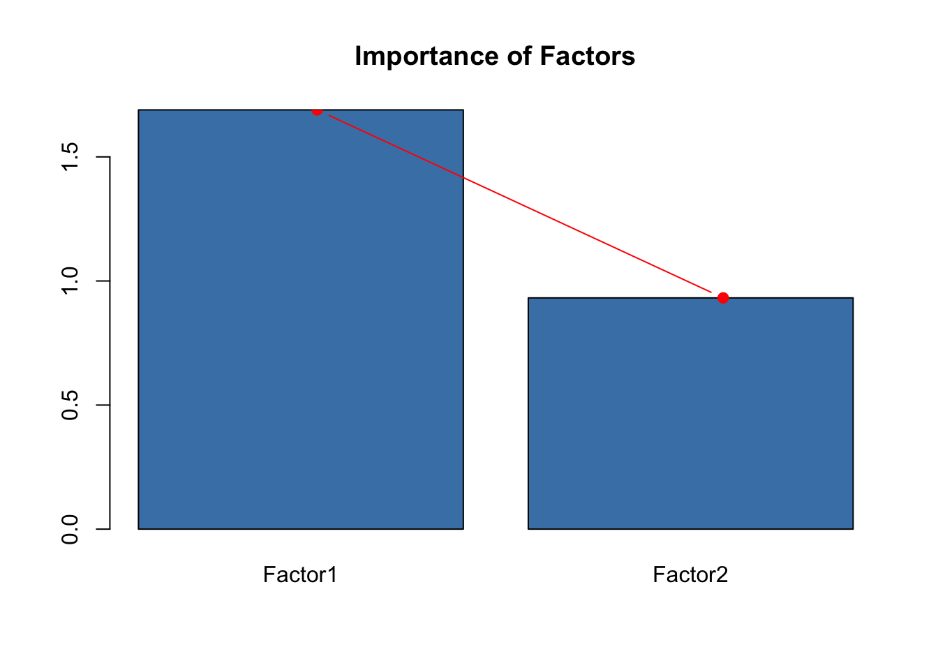
We do not worry too much that the cumulative proportion of variance explained is lower than 80% here: we are trying to analyze underlying factors rather than finding subspaces maximizing the variance, so this is to be expected.
Likelihood ratio test
The final part of the factanal() output shows the performance of the model in the likelyhood ratio test, which is possible because the factors are computed using a maximum likelihood estimate. Likelihood ratio test is a hypothesis test with respect to the following null hypothesis:
- \(H_0\): 2 factors are enough to capture the information contained in the data set.
Usually, we reject \(H_0\) when the p value is small enough (<0.05), and we do not reject it otherwise. If we reject \(H_0\), we are implying that we need to account for more factors; if we fail to reject \(H_0\) (as in our case above) then it is very likely that there are enough factors for the model to be appropriate.
Visualization
To visualize our data in the space of factors, we need to determine the scores.
library(ggfortify)
life.fa <- factanal(dat[,-(1:8)], factors = 2, scores = 'regression')
autoplot(life.fa, data = dat, colour = 'Life.expectancy')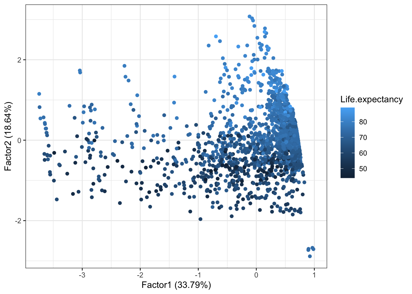
Then we add loadings and labels
autoplot(life.fa, data = dat, colour = 'Life.expectancy',
loadings = TRUE, loadings.label = TRUE, loadings.label.size  = 3)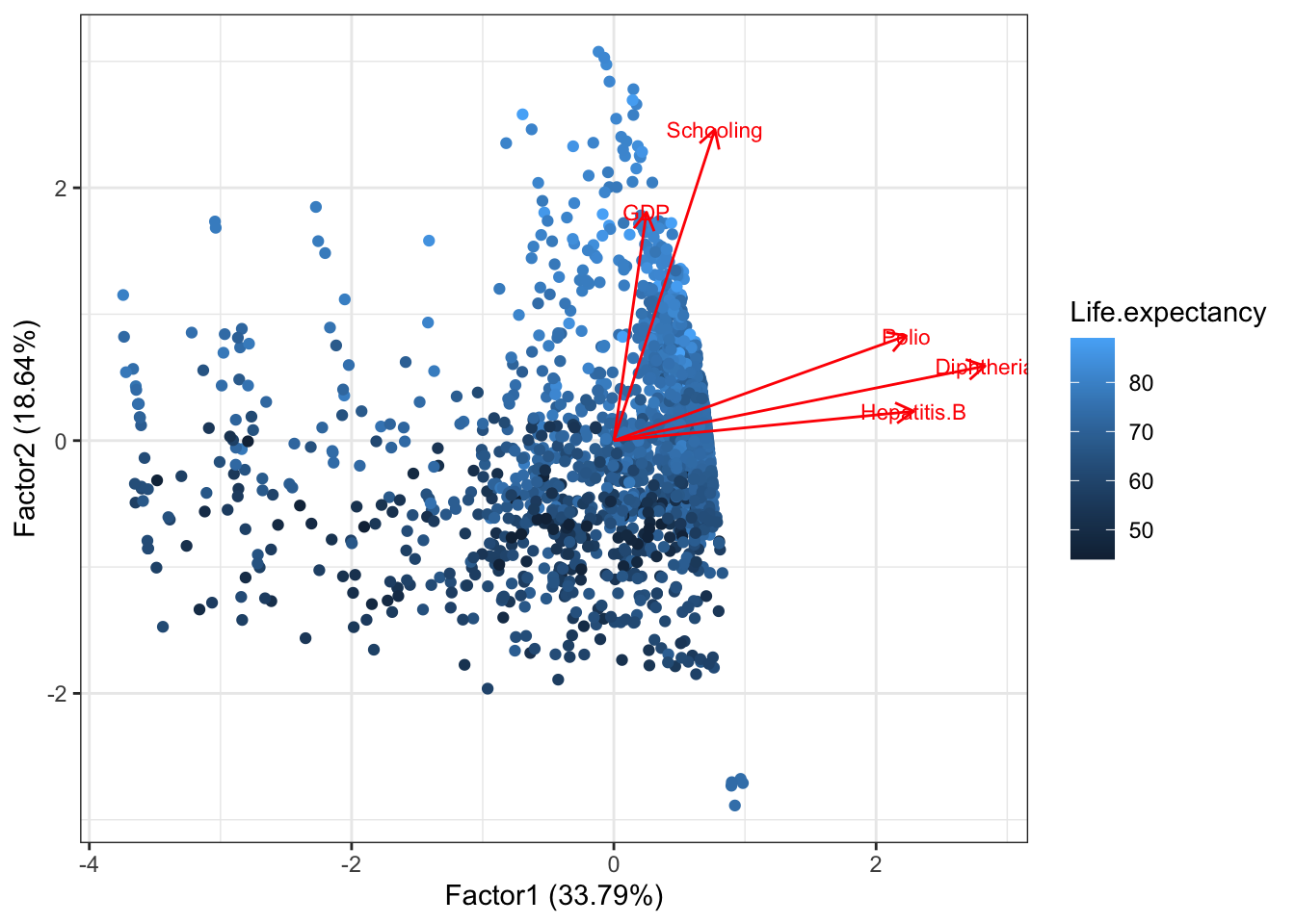
More variables
If we want to account for more variables, then we need more factors. We can check this on the likelihood ratio tests:
factanal(dat[,-c(1,2,3,5,7,8)], factors = 2)##
## Call:
## factanal(x = dat[, -c(1, 2, 3, 5, 7, 8)], factors = 2)
##
## Uniquenesses:
## Adult.Mortality under.five.deaths Hepatitis.B Polio Diphtheria GDP
## 0.734 0.914 0.514 0.491 0.270 0.741
## Schooling
## 0.315
##
## Loadings:
## Factor1 Factor2
## Adult.Mortality -0.141 -0.496
## under.five.deaths -0.215 -0.199
## Hepatitis.B 0.692
## Polio 0.669 0.247
## Diphtheria 0.835 0.181
## GDP 0.503
## Schooling 0.214 0.800
##
## Factor1 Factor2
## SS loadings 1.742 1.278
## Proportion Var 0.249 0.183
## Cumulative Var 0.249 0.432
##
## Test of the hypothesis that 2 factors are sufficient.
## The chi square statistic is 49.46 on 8 degrees of freedom.
## The p-value is 5.19e-08factanal(dat[,-c(1,2,3,5,7,8)], factors = 3)##
## Call:
## factanal(x = dat[, -c(1, 2, 3, 5, 7, 8)], factors = 3)
##
## Uniquenesses:
## Adult.Mortality under.five.deaths Hepatitis.B Polio Diphtheria GDP
## 0.715 0.005 0.516 0.496 0.247 0.728
## Schooling
## 0.353
##
## Loadings:
## Factor1 Factor2 Factor3
## Adult.Mortality -0.136 -0.516
## under.five.deaths -0.152 -0.106 0.980
## Hepatitis.B 0.678 -0.139
## Polio 0.660 0.255
## Diphtheria 0.847 0.188
## GDP 0.515
## Schooling 0.206 0.769 -0.115
##
## Factor1 Factor2 Factor3
## SS loadings 1.701 1.239 0.999
## Proportion Var 0.243 0.177 0.143
## Cumulative Var 0.243 0.420 0.563
##
## Test of the hypothesis that 3 factors are sufficient.
## The chi square statistic is 1.49 on 3 degrees of freedom.
## The p-value is 0.684While two factors are too few, there is a high probability (\(p=0.684\)) that three factors are appropriate to model our data frame with 7 variables.
life2.fa <- factanal(dat[,-c(1,2,3,5,7,8)], factors = 3, scores = 'regression')Let us check the output of this new analysis:
Uniquenesses show that a good portion of variance is accounted by the model for
under 5 deaths,Diphtheriaimmunization andSchooling, while the model fails to account for most of the variance ofAdult mortalityandGDP. This does not mean that these variables don’t play a role, though, as the factor model aims at explaining covariances too.Loadings show that the first factor is a combination mostly of immunization rates, the second factor has a mixed contribution accounting positively for socioeconomical factors and negatively for mortality factors (so, “wealth with effective death prevention” could be a label for this factor) and the third factor predominantly represents
under 5 deaths(possible label: “adjusted infant mortality”).Together, the three factors explain \(56.3 \%\) of the total variance, which is a fair amount given that we’re working with a factor model rather than with PCA.
L <- life2.fa$loadings
SS <- apply(L^2, 2, sum)
barplot(SS, col='steelblue' , main="Importance of Factors")
lines(x = c(.75,2,3.25), SS, type="b", pch=19, col = "red")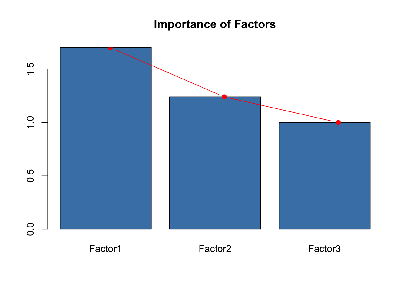
To see how good is the model at representing covariances, we can compute the residual matrix. This is the difference between the covariance \(\Sigma_X\) estimated by the model and the observed correlation matrix.
Sigmae <- diag(life2.fa$uniquenesses)
SigmaX <- L %*% t(L) + Sigmae
S <- life2.fa$correlation
round(S - SigmaX,5)
## Adult.Mortality under.five.deaths Hepatitis.B Polio Diphtheria GDP Schooling
## Adult.Mortality 0.00000 -1e-05 -0.00705 -0.00257 0.00369 0.00112 -0.00069
## under.five.deaths -0.00001 0e+00 0.00000 0.00000 0.00000 -0.00001 0.00000
## Hepatitis.B -0.00705 0e+00 0.00000 -0.00111 0.00008 -0.01154 0.00164
## Polio -0.00257 0e+00 -0.00111 0.00001 0.00034 -0.00281 -0.00001
## Diphtheria 0.00369 0e+00 0.00008 0.00034 0.00000 0.00548 -0.00064
## GDP 0.00112 -1e-05 -0.01154 -0.00281 0.00548 -0.00001 -0.00028
## Schooling -0.00069 0e+00 0.00164 -0.00001 -0.00064 -0.00028 0.00000Visualization is a bit more challenging, as we have 3 factors to account for. A first method is to plot 2 factors at a time. We can do this using autoplot
autoplot(life2.fa, data = dat, colour = 'Life.expectancy')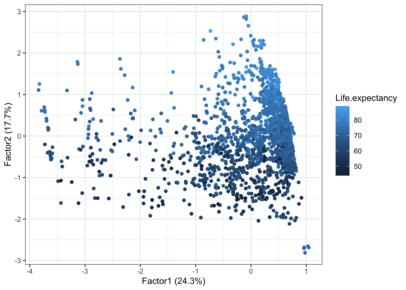 Both factor 1 and factor 2 seem to contribute to life expectancy.
The contribution of factor 3 is less clear, as most data points are positioned low (meaning that most coutries have a low death rate for under 5).
autoplot(life2.fa,x=1, y=3,data = dat, colour = 'Life.expectancy')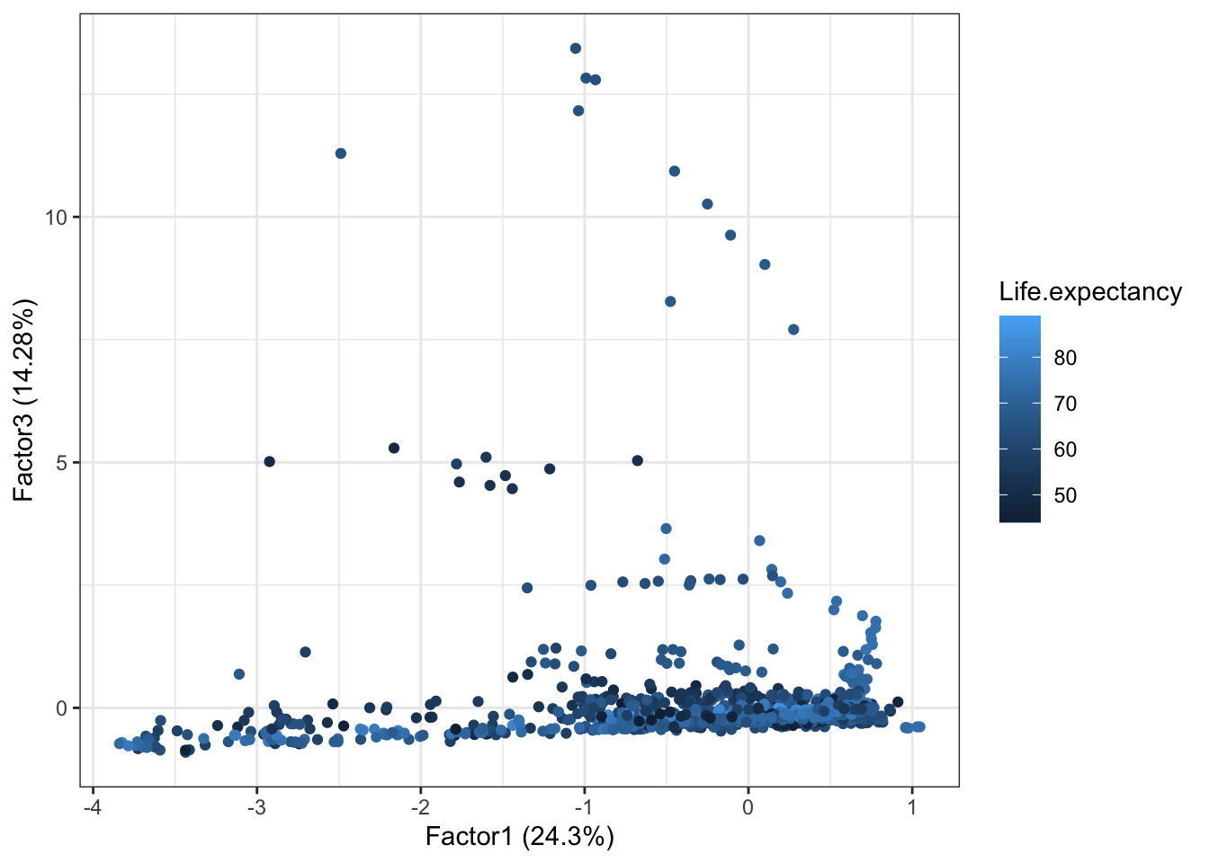
We can still remark that even countries with low Factor3 can have a low life expectancy, meaning that Factor3 contribution alone is not very significant.
Plotting Factor 2 against Factor 3 completes the picture of the relationships between the different factors.
autoplot(life2.fa,x=2, y=3,data = dat, colour = 'Life.expectancy')
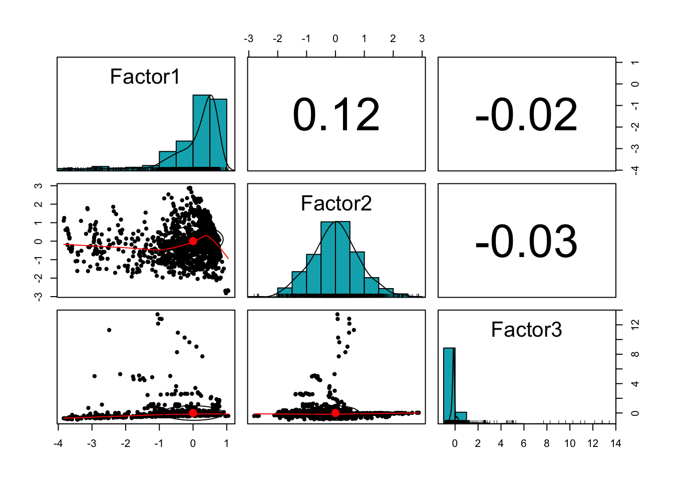
If we want all three pictures in a single visualization, our good old friend, the scatterplot matrix is the right choice
life2.scores <- as.data.frame(life2.fa$scores)
library(psych)
pairs.panels(life2.scores,
             method = "pearson", # correlation method
             hist.col = "#00AFBB",
             density = TRUE,  # show density plots
             )
Finally, given the greater importance of Factors 1 and 2, and the difference in scale of Factor 3, it might make sense to visualize our picture using a bubble plot, where Factor 3 is accounted on the size of the points
#installpackages('plotly')
library(plotly)
plot_ly(life2.scores, x=~Factor1, y=~Factor2, size=~Factor3,
        sizes = c(1,25), type='scatter', mode='markers', marker = list(opacity = 0.5, sizemode = "diameter"))
Less countries?
The data we analyzed has a high complexity: not only it measures 11 numerical variables, but contains \(>1500\) observations! After a first exploratory analysis, we notice that there is a marked difference in behaviour between some of these observations: most notably, between the countries with high development and those with medium to low development. It seems reasonable to perform separated analysis for different kinds of countries. We begin by selecting those observations with lowest life expectancy.
newdat <- dat[dat$Life.expectancy< 65,]
factanal(newdat[,-c(1,2,3,5,7,8)], factors = 3)
##
## Call:
## factanal(x = newdat[, -c(1, 2, 3, 5, 7, 8)], factors = 3)
##
## Uniquenesses:
## Adult.Mortality under.five.deaths Hepatitis.B Polio Diphtheria GDP
## 0.899 0.005 0.411 0.607 0.120 0.573
## Schooling
## 0.542
##
## Loadings:
## Factor1 Factor2 Factor3
## Adult.Mortality 0.311
## under.five.deaths -0.168 0.981
## Hepatitis.B 0.745 -0.153
## Polio 0.616
## Diphtheria 0.932 0.107
## GDP 0.652
## Schooling 0.137 0.662
##
## Factor1 Factor2 Factor3
## SS loadings 1.855 0.995 0.993
## Proportion Var 0.265 0.142 0.142
## Cumulative Var 0.265 0.407 0.549
##
## Test of the hypothesis that 3 factors are sufficient.
## The chi square statistic is 2.01 on 3 degrees of freedom.
## The p-value is 0.57What do we remark?
- \(p\)-value is slightly lower: selecting less data does not improve the fitness of the model
- Uniquenesses show that a good portion of variance is accounted by
the model for
under 5 deathsandDiphtheriaimmunization (as in the previous model), while the model fails to account for most of the variance ofAdult mortality.Polio,GDP, andSchoolingare somewhere in the middle. - The model is quite similar to the one with all data points, but now Factor 2 and Factor 3 are exchanged!
life3.fa <- factanal(newdat[,-c(1,2,3,5,7,8)], factors = 3, scores = 'regression')
life3.scores <- as.data.frame(life3.fa$scores)
plot_ly(life3.scores, x=~Factor1, y=~Factor3, size=~Factor2,
        sizes = c(1,25), type='scatter', mode='markers', marker = list(opacity = 0.5, sizemode = "diameter"))
## Warning: `line.width` does not currently support multiple values.