Lab 4: Factor Analysis
Lab 4: Factor Analysis
This computer practical consists of three exercises.
- In exercise 1, you will perform Factor Analysis on a climate data set;
- In exercise 2, you will explore further techniques on the interpretation of the factors;
- In exercise 3, you will use the command fa() and compare it with factanal().
Exercise 1 (French climate)
The following data set was created by researchers at Freie Universit"at in Berlin to illustrate dimension reduction techniques. It contains 36 observations of 12 variables related to climate in different locations of France. We need to preprocess it to uniformize format and treat some of the variables as numerical.
clim <- read.csv("https://userpage.fu-berlin.de/soga/data/raw-data/Climfrance.csv", sep = ";")
clim[, "p_mean"] <- as.numeric(gsub(",", "", clim[, "p_mean"]))
clim[, "altitude"] <- as.numeric(gsub(",", "", clim[, "altitude"]))
newclim <- clim[,-1]
Task 1a
Perform FA on the data setnewclim with 2 and 3 factors,
and interpret uniquesnesses, loadings, and likelihood ratio test.
Discuss the differences between the two models obtained.Solution to Task 1a
Click for solution
clim.fa2 <- factanal(newclim, factors = 2, scores="regression")
clim.fa3 <- factanal(newclim, factors = 3, scores="regression")
We first analyze the model with two factors
clim.fa2##
## Call:
## factanal(x = newclim, factors = 2, scores = "regression")
##
## Uniquenesses:
## altitude lat lon t_mean t_max t_min
## 0.099 0.240 0.777 0.006 0.332 0.205
## relhumidity p_mean p_max24h rainydays sun_shine_hperyrs
## 0.335 0.974 0.433 0.221 0.219
##
## Loadings:
## Factor1 Factor2
## altitude 0.159 -0.936
## lat -0.869
## lon 0.472
## t_mean 0.247 0.966
## t_max 0.152 0.803
## t_min 0.287 0.844
## relhumidity -0.815
## p_mean -0.158
## p_max24h 0.740 0.139
## rainydays -0.849 -0.242
## sun_shine_hperyrs 0.879
##
## Factor1 Factor2
## SS loadings 3.877 3.283
## Proportion Var 0.352 0.298
## Cumulative Var 0.352 0.651
##
## Test of the hypothesis that 2 factors are sufficient.
## The chi square statistic is 128.72 on 34 degrees of freedom.
## The p-value is 6.13e-13The likelihood ratio test indicates that the model with 2 factors is
very unlikely to be accurate. This means that the analysis provided will
not be sound, but it can still be valid to explore pattern in the data.
Uniquenesses tell us that this model will not encode meaningfully the
variance of precipitation mean and longitude,
but by contrast it will encode well the variance of variables such as
altitude, temperature mean, and to some extent
latitude, min temperature,
sunshine hours and rainy days. The cumulative
variance explained by the two factors is \(65.1\%\), sufficiently high to make it
worthwhile to look at this model, even though it is a hypersimplified
one.
Looking at the loadings one can attempt an interpretation of the factors:
- Factor 1 has positive contributions from sunshine hours and daily precipitations and negative contributions from latitude, humidity and rainy days. A labeling of this factor is challenging (see exercise 2 to see how to improve the interpretation of factors using rotations), but a fair attempt could be “general dryness”, noting that lower latitudes correspond to towns where humidity is lower, precipitations are rarer but also more substantial.
- Factor 2 is somewhat easier to interpret: it is essentially a weighted measure of temperatures (altitude being negatively correlated with temperatures).
clim.fa3##
## Call:
## factanal(x = newclim, factors = 3, scores = "regression")
##
## Uniquenesses:
## altitude lat lon t_mean t_max t_min
## 0.075 0.005 0.608 0.005 0.302 0.184
## relhumidity p_mean p_max24h rainydays sun_shine_hperyrs
## 0.380 0.630 0.459 0.005 0.234
##
## Loadings:
## Factor1 Factor2 Factor3
## altitude 0.207 -0.919 0.193
## lat -0.941 -0.331
## lon 0.435 -0.450
## t_mean 0.209 0.973
## t_max 0.124 0.819 0.108
## t_min 0.231 0.844 -0.224
## relhumidity -0.782
## p_mean -0.113 0.595
## p_max24h 0.706 0.182
## rainydays -0.863 -0.238 0.441
## sun_shine_hperyrs 0.850 0.120 -0.169
##
## Factor1 Factor2 Factor3
## SS loadings 3.810 3.293 1.010
## Proportion Var 0.346 0.299 0.092
## Cumulative Var 0.346 0.646 0.738
##
## Test of the hypothesis that 3 factors are sufficient.
## The chi square statistic is 84.32 on 25 degrees of freedom.
## The p-value is 2.37e-08With respect to the one with 2 factors, the factor analysis with 3 factors is:
- More accurate (higher \(p\)-value in the likelihood ratio test) but still not very precise, so good only for exploration.
- Variance of
precipitation meanandlongitudeare better accounted for and more generally a cumulative proportion of variance of \(73.8 \%\) is explained by the model, which is very good given that we are doing FA rather than PCA. - Loadings show that Factor 1 and Factor 2 are very similar to the previous model, Factor 3 is mildly associated with “rainy weather”, where the mean precipitation and the number of rainy days count more than the maximum precipitation in 24hours. This is the kind of rain more typically associated with proximity with the ocean
Task 1b
Plot the loadings and the scores from the factor analysis with 2 factors.
Click for hint
Use autoplot() for plotting the scores, and plot()Click for solution
As we saw in the workshop, the scores can be plotted using the
autoplot() command. Here we scale the plot to get a more
faithful representation
library(ggfortify)
sp <- autoplot(clim.fa2, data = clim, col="blue")
sp + expand_limits(x=c(-3.5,3.5), y=c(-4.5, 2))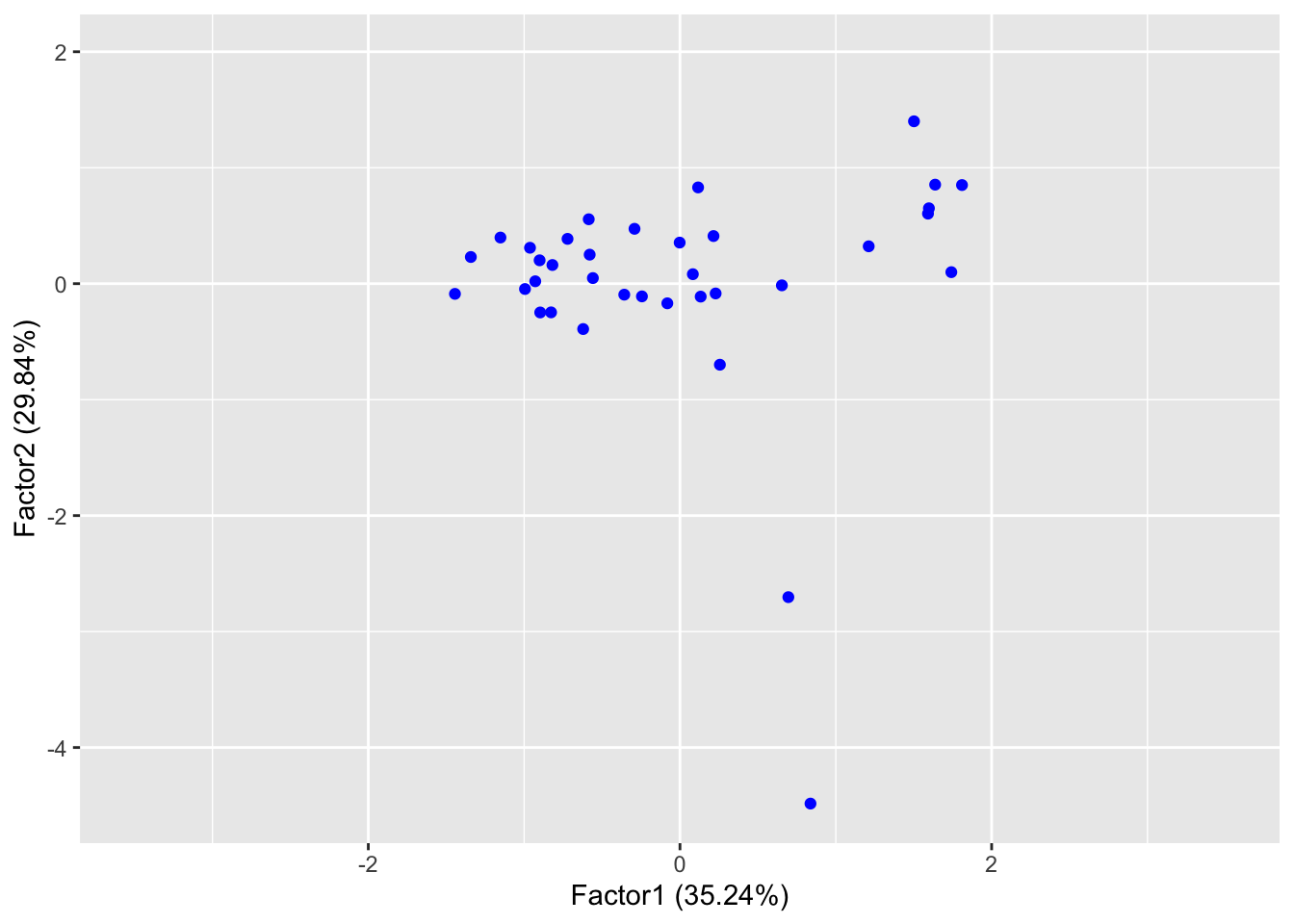
If we want to add loadings to the plot, we can do it as in the case of PCA:
library(ggfortify)
spl <- autoplot(clim.fa2, data = clim, col="blue", repel=TRUE, loadings=TRUE, loadings.label=TRUE)
spl + expand_limits(x=c(-3.5,3.5), y=c(-4.5, 2))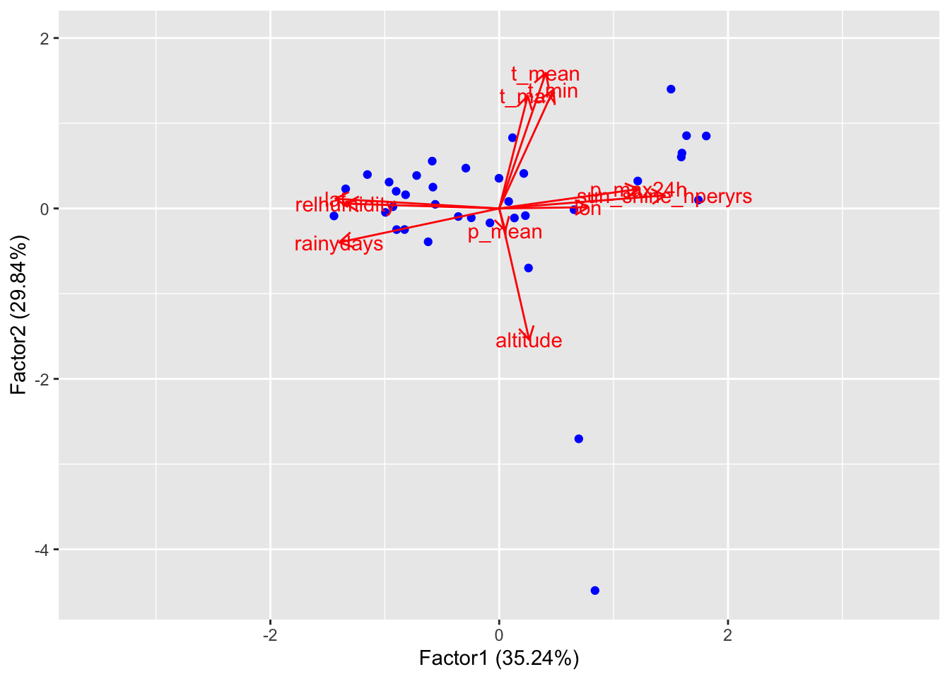
It is easy to see that the variance on Factor 1 is more homogeneous,
while on Factor 2 it is mostly explained by the presence of outliers.
Variation in temperatures is due mostly on the altitude of the different
stations, while variation in “general dryness” is a more interesting
factor. We can add labels to scores to see how different locations
perform:
library(ggfortify)
rownames(clim) <- clim$station
autoplot(clim.fa2, data = clim, col="blue", label=TRUE, repel=TRUE)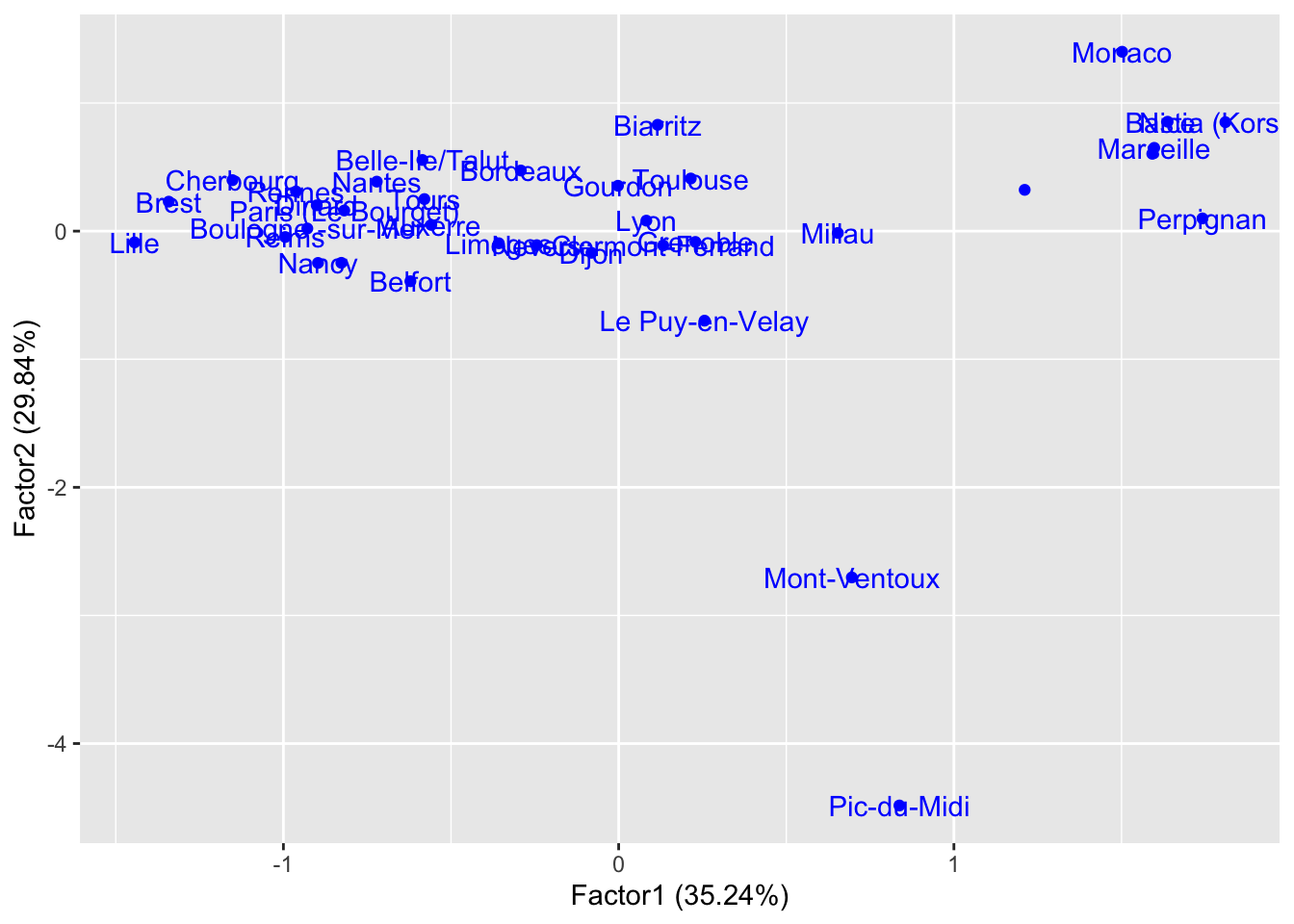 Perpignan, Marseille, and Bastia are the most generally dry, while
Lille, Brest, and Cherbourg are the most generally wet. We realize in
this way that Factor 1 is a very good indicator of “being next to the
Mediterrenean Sea”.
Perpignan, Marseille, and Bastia are the most generally dry, while
Lille, Brest, and Cherbourg are the most generally wet. We realize in
this way that Factor 1 is a very good indicator of “being next to the
Mediterrenean Sea”.
It turns out that 4 factors might be more appropriate to explain our
model (see Task 3a). This can be checked with a likelihood ratio test,
but also by performing PCA and checking a screeplot of the variance
explained by the principal components.
Task 1c
Perform FA with 4 factors on the climate data and try to come up with a way to effectively visualize your results.
Hint: if you need ideas, check the Lecture 5 of the first part of the module
Click for solution
clim.fa4 <- factanal(newclim, factors = 4, scores="regression")The first thing to try is a scatterplot matrix, plotting pairwise all factors against each other.
clim4.scores <- as.data.frame(clim.fa4$scores)
library(psych)
pairs.panels(clim4.scores,
             method = "pearson", # correlation method
             hist.col = "#00AFBB"
             )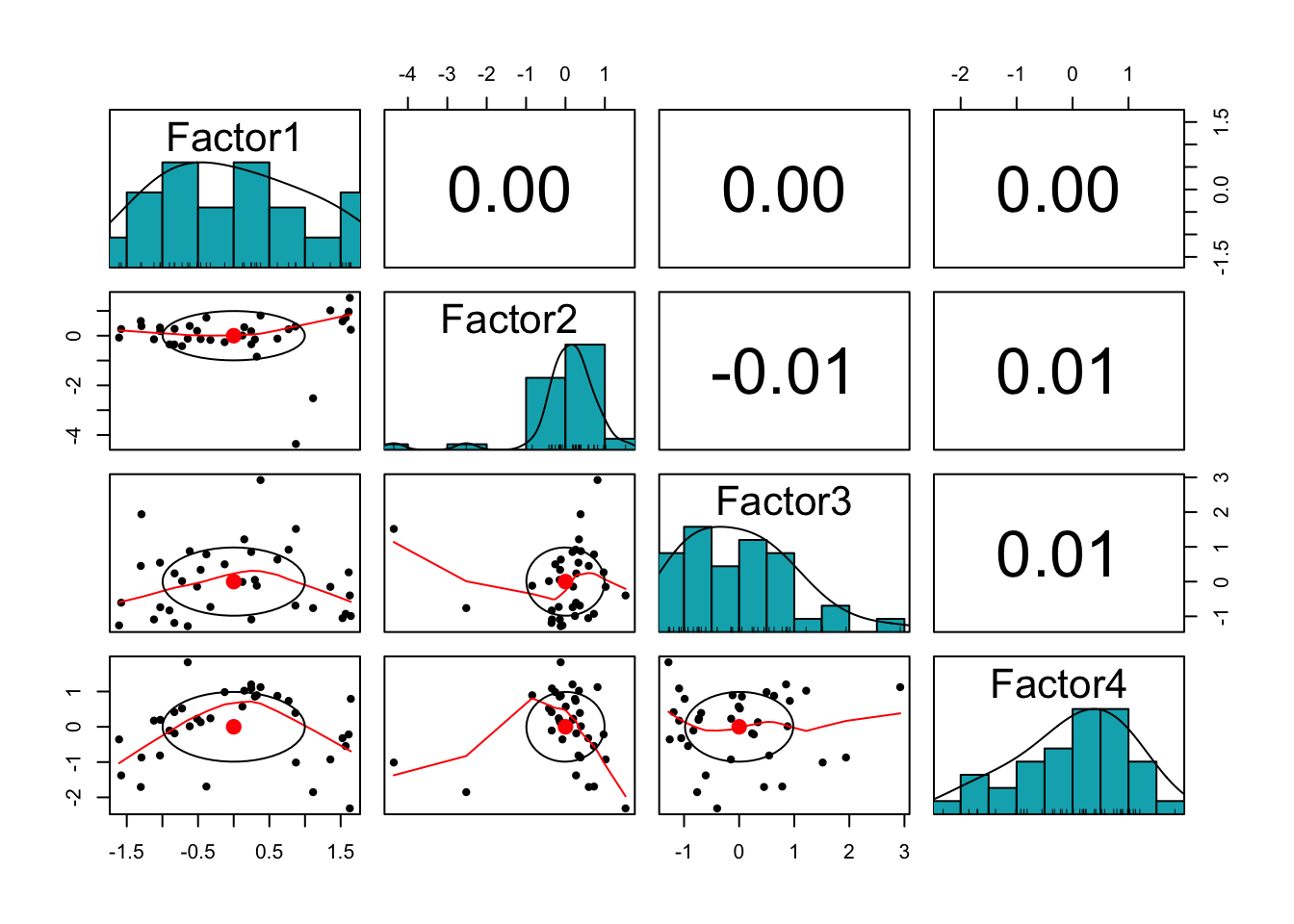
To supplement this, we can use a bubble plot, explaining two extra dimensions using colour and dimension of the bubbles. If you choose to do so, you will need to associate factors with explanating features. One idea, is to use position in the plane for those factors that are less skewed (e.g. Factor 1 in the previous plot) and non-positional features for those factors that are more skewed (e.g. Factor 2 in the previous plot).
summary(clim.fa4$scores)## Factor1 Factor2 Factor3 Factor4
## Min. :-1.607874 Min. :-4.3595 Min. :-1.28297 Min. :-2.3126
## 1st Qu.:-0.829780 1st Qu.:-0.1542 1st Qu.:-0.77915 1st Qu.:-0.6122
## Median :-0.002424 Median : 0.1886 Median :-0.06458 Median : 0.1863
## Mean : 0.000000 Mean : 0.0000 Mean : 0.00000 Mean : 0.0000
## 3rd Qu.: 0.793715 3rd Qu.: 0.3855 3rd Qu.: 0.56700 3rd Qu.: 0.8086
## Max. : 1.642677 Max. : 1.5249 Max. : 2.92347 Max. : 1.8299From this summary we see that factors 1 and 3 have similar median and mean, while for factors 2 and 4 they are quite different. We then choose to associate colour with Factor 2 and size with Factor 4.
library(plotly)
plot_ly(clim4.scores, x=~Factor1, y=~Factor3, size=~Factor4, color=~Factor2,
        sizes = c(1,50), type='scatter', mode='markers', marker = list(opacity = 0.5, sizemode = "diameter"), label=TRUE)
Of course, these are not the only possibilities: other instances of scatterplot matrices, as well as parallel plots are all good choices to get more insight of your data set.
If you are interested in how particular places perform on these 4 factors you can even try out glyphs!
palette(rainbow(12,s=0.7,v=0.75))
stars(clim4.scores[1:6,], labels=(clim$station[1:6]), draw.segments=TRUE)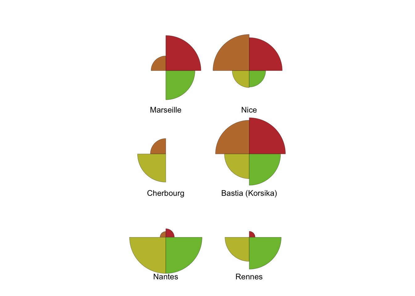
Exercise 2 (Factor interpretation and rotation)
One aspect of Factor Analysis that we did not consider is the fact that we can apply a rotation to the space of factors without changing the main features of the model: the uniquenesses will be the same, as well as the proportion of variance explained. However, rotating the space might be useful to find a better interpretation of factors. There are infinitely many way of producing a rotation: the command factanal() has built-in standard methods that allow one to easily check the most relevant ones.
Rather than using real-world data, in this exercise you’ll generate a data set from a multivariate normal distribution.
Recall from Lab2 how to generate observations of p variables from a multivariate normal distribution with correlation matrix given as \(corr(x_{i},x_{j}) = \rho^{|i-j|}\). We’ll set \(p=13\) and generate \(n=200\) observations in the case \(\rho=0.92\).
covmat <- function(rho, p) {
  rho^(abs(outer(seq(p), seq(p), "-")))
}
library(MASS)
set.seed(123)
p = 13
n = 200
cov.e = covmat(0.92, p)
mean.e = rep(0, p)
dd <- mvrnorm(n, mean.e, cov.e)
Task 2a
Suppose we want to perform Factor Analysis on our data set
dd. Determine an appropriate number of factors to use by
performing PCA. Even though the principal components are not the same in
PCA and FA, the number of appropriate components in both cases is often
equal, so this makes sense.
Click for solution
prr <- prcomp(dd)
summary(prr)
## Importance of components:
## PC1 PC2 PC3 PC4 PC5 PC6 PC7 PC8 PC9 PC10 PC11
## Standard deviation 2.8938 1.3769 0.77405 0.57375 0.44908 0.37321 0.28752 0.25974 0.24622 0.23526 0.2044
## Proportion of Variance 0.7025 0.1590 0.05027 0.02762 0.01692 0.01169 0.00694 0.00566 0.00509 0.00464 0.0035
## Cumulative Proportion 0.7025 0.8616 0.91185 0.93946 0.95638 0.96807 0.97500 0.98066 0.98575 0.99039 0.9939
## PC12 PC13
## Standard deviation 0.20089 0.17998
## Proportion of Variance 0.00339 0.00272
## Cumulative Proportion 0.99728 1.00000plot(summary(prr)$importance[2,], type="b", xlab="PCs", ylab="Variability explained")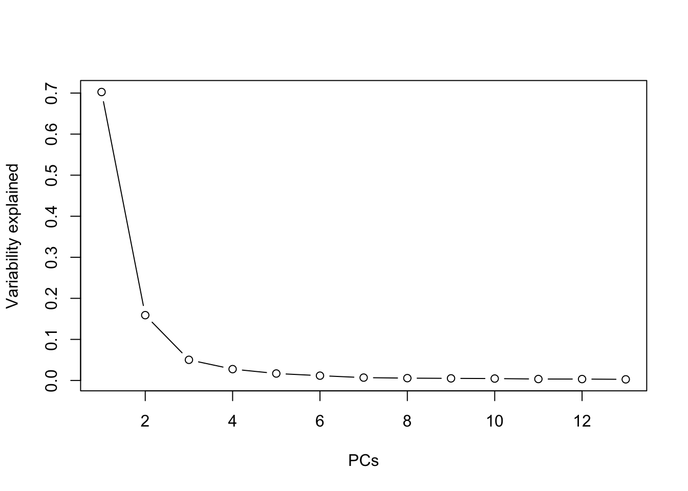 Two components explain \(>86\%\) of
the variance, and one can see an “elbow” at 3 components, so 2 or 3 are
both appropriate choices.
Two components explain \(>86\%\) of
the variance, and one can see an “elbow” at 3 components, so 2 or 3 are
both appropriate choices.
Task 2b
Apply factor analysis using the chosen number of factors, and plot loadings and scores.
Click for solution
norm.fa <- factanal(dd, factors = 3, scores="regression")
norm.fa
##
## Call:
## factanal(x = dd, factors = 3, scores = "regression")
##
## Uniquenesses:
## [1] 0.233 0.102 0.067 0.114 0.166 0.128 0.063 0.087 0.093 0.091 0.044 0.114 0.238
##
## Loadings:
## Factor1 Factor2 Factor3
## [1,] 0.158 0.849 0.145
## [2,] 0.234 0.906 0.151
## [3,] 0.231 0.906 0.243
## [4,] 0.254 0.831 0.362
## [5,] 0.305 0.711 0.485
## [6,] 0.374 0.576 0.632
## [7,] 0.453 0.462 0.720
## [8,] 0.599 0.370 0.646
## [9,] 0.713 0.295 0.558
## [10,] 0.835 0.228 0.399
## [11,] 0.924 0.218 0.234
## [12,] 0.893 0.238 0.178
## [13,] 0.830 0.225 0.153
##
## Factor1 Factor2 Factor3
## SS loadings 4.540 4.534 2.385
## Proportion Var 0.349 0.349 0.183
## Cumulative Var 0.349 0.698 0.881
##
## Test of the hypothesis that 3 factors are sufficient.
## The chi square statistic is 452.45 on 42 degrees of freedom.
## The p-value is 3.13e-70As expected, uniquenesses are similar for all features. A big proportion of the variance is explained, but the likelihood ratio test is inconclusive.
Let us plot scores and loadings against the first two factors
autoplot(norm.fa, loadings=TRUE, loadings.label=TRUE)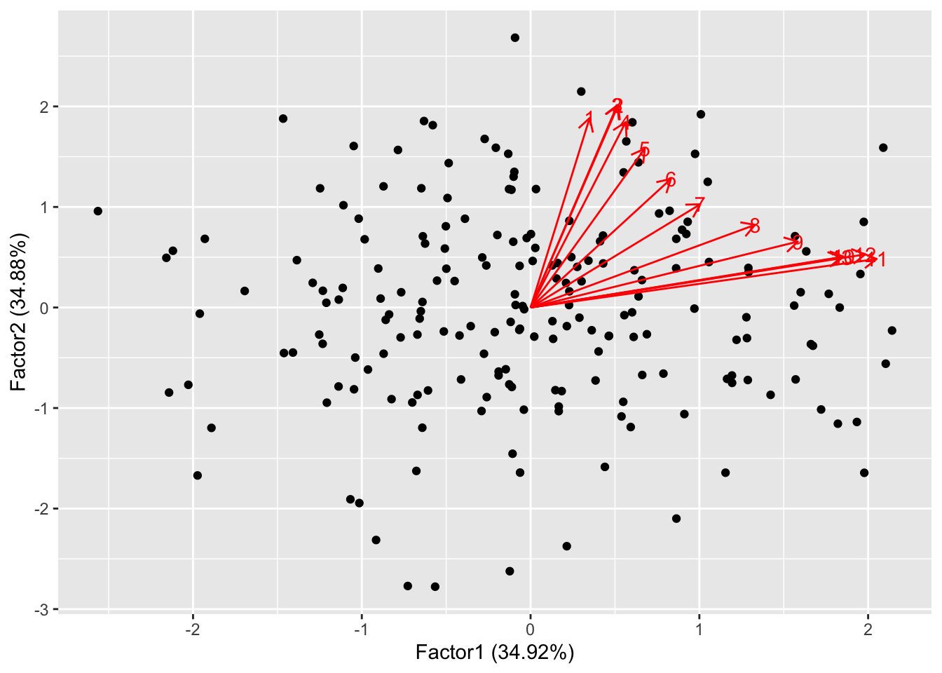 The data points are scattered quite uniformly in the space. The loadings
are all in the first quadrant and are anticlockwise ordered. This is
because, by design, the first few features (that are highly correlated)
contribute the most to the first factor, while the last features
contribute most to the second factor. This behaviour is quite similar to
what happens for PCA:
The data points are scattered quite uniformly in the space. The loadings
are all in the first quadrant and are anticlockwise ordered. This is
because, by design, the first few features (that are highly correlated)
contribute the most to the first factor, while the last features
contribute most to the second factor. This behaviour is quite similar to
what happens for PCA:
autoplot(prr, loadings=TRUE, loadings.label=TRUE)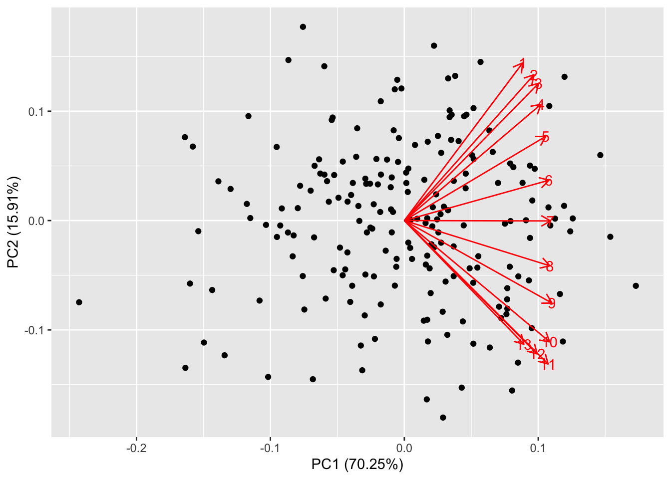
We saw that our factors are created with the aim to account for most of
the variability in the data. One issue arising from this is that
sometimes different factors tend to load portions of the same variables,
while it would be desirable for different factors to load different
variables, if possible.
The solution to this problem is to apply a rotation to the matrix of
loadings. This is perfectly acceptable, as it does not affect
uniquenesses and the fitness of the model. However, loadings get
repositioned to help maximize interpretability. In factanal()
this is controlled via the option rotation:
norm.fa.none <- factanal(dd, factors = 3, rotation = "none")
norm.fa.varimax <- factanal(dd, factors = 3, rotation = "varimax")
norm.fa.promax <- factanal(dd, factors = 3, rotation = "promax")
Task 2c
Compare the above rotation patterns graphically by plotting the loadings in the three situations above. Comment on which rotation gives a better interpretation of the factors
Solution to task 2c
Click for solution
par(mfrow = c(1, 3))
plot(norm.fa.none$loadings[, 1],
norm.fa.none$loadings[, 2],
xlab = "Factor 1",
ylab = "Factor 2",
ylim = c(-1, 1),
xlim = c(-1, 1),
col= "blue",
main = "No rotation")
abline(h = 0, v = 0)
plot(norm.fa.varimax$loadings[, 1],
norm.fa.varimax$loadings[, 2],
xlab = "Factor 1",
ylab = "Factor 2",
ylim = c(-1, 1),
xlim = c(-1, 1),
col= "blue",
main = "Varimax rotation")
abline(h = 0, v = 0)
plot(norm.fa.promax$loadings[, 1],
norm.fa.promax$loadings[, 2],
xlab = "Factor 1",
ylab = "Factor 2",
ylim = c(-1, 1),
xlim = c(-1, 1),
col= "blue",
main = "Promax rotation")
abline(h = 0, v = 0)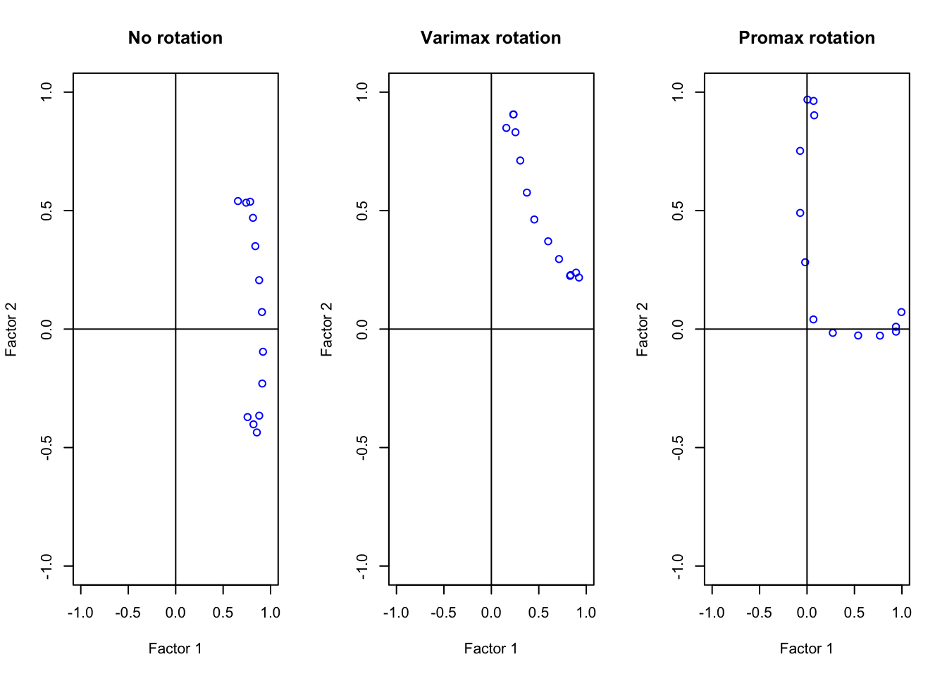 The promax rotation is clearly the best method. Our variables are either
highly contributing to Factor 1 or to Factor 2 but not both! To check
this, look at the factor analysis summary:
The promax rotation is clearly the best method. Our variables are either
highly contributing to Factor 1 or to Factor 2 but not both! To check
this, look at the factor analysis summary:
norm.fa.promax##
## Call:
## factanal(x = dd, factors = 3, rotation = "promax")
##
## Uniquenesses:
## [1] 0.233 0.102 0.067 0.114 0.166 0.128 0.063 0.087 0.093 0.091 0.044 0.114 0.238
##
## Loadings:
## Factor1 Factor2 Factor3
## [1,] 0.938
## [2,] 0.995 -0.120
## [3,] 0.937
## [4,] 0.768 0.247
## [5,] 0.539 0.472
## [6,] 0.272 0.736
## [7,] 0.891
## [8,] 0.282 0.750
## [9,] 0.490 0.590
## [10,] 0.752 0.308
## [11,] 0.968
## [12,] 0.963
## [13,] 0.902
##
## Factor1 Factor2 Factor3
## SS loadings 3.729 3.573 2.663
## Proportion Var 0.287 0.275 0.205
## Cumulative Var 0.287 0.562 0.767
##
## Factor Correlations:
## Factor1 Factor2 Factor3
## Factor1 1.000 0.692 0.701
## Factor2 0.692 1.000 0.467
## Factor3 0.701 0.467 1.000
##
## Test of the hypothesis that 3 factors are sufficient.
## The chi square statistic is 452.45 on 42 degrees of freedom.
## The p-value is 3.13e-70
Exercise 3
In this exercise, you’ll use the same climate data set of Exercise 1.
This time, you’ll explore how to perform factor analysis using the
fa() command.
Task 3a
Determine the number of factors you should use to perform FA.
Click for solution
clim.pca <- prcomp(newclim)
summary(clim.pca)
## Importance of components:
## PC1 PC2 PC3 PC4 PC5 PC6 PC7 PC8 PC9 PC10
## Standard deviation 505.8372 335.3215 188.32413 28.92650 16.19531 3.51162 2.54052 1.80821 1.58573 0.6494
## Proportion of Variance 0.6319 0.2777 0.08759 0.00207 0.00065 0.00003 0.00002 0.00001 0.00001 0.0000
## Cumulative Proportion 0.6319 0.9096 0.99722 0.99929 0.99994 0.99997 0.99998 0.99999 1.00000 1.0000
## PC11
## Standard deviation 0.4282
## Proportion of Variance 0.0000
## Cumulative Proportion 1.0000plot(summary(clim.pca)$importance[2,], type="b", xlab="PCs", ylab="Variability explained")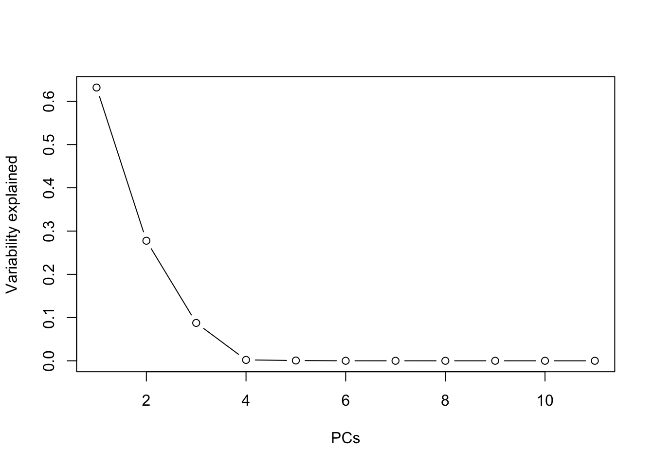 Four factors are the ideal choice, while two or three factors give
already a good idea (confirming our findings in Ex. 1).
Four factors are the ideal choice, while two or three factors give
already a good idea (confirming our findings in Ex. 1).
You can now proceed to the factor analysis. This is done
#install.packages('GPArotation')
library(GPArotation)
clim.fa <- fa(newclim, nfactors = 4)
Task 3b
Explore the output of fa() and compare with
factanal()
Click for solution
We first check the structure of our output:
str(clim.fa)## List of 52
## $ residual : num [1:11, 1:11] 0.0449 -0.0453 -0.0204 0.0172 -0.0054 ...
## ..- attr(*, "dimnames")=List of 2
## .. ..$ : chr [1:11] "altitude" "lat" "lon" "t_mean" ...
## .. ..$ : chr [1:11] "altitude" "lat" "lon" "t_mean" ...
## $ dof : num 17
## $ chi : num 3.78
## $ nh : num 36
## $ rms : num 0.0309
## $ EPVAL : num 1
## $ crms : num 0.0556
## $ EBIC : num -57.1
## $ ESABIC : num -4.03
## $ fit : num 0.978
## $ fit.off : num 0.995
## $ sd : num 0.0294
## $ factors : num 4
## $ complexity : Named num [1:11] 1.16 1.33 1.87 1.05 1.47 ...
## ..- attr(*, "names")= chr [1:11] "altitude" "lat" "lon" "t_mean" ...
## $ n.obs : int 36
## $ objective : num 2.2
## $ criteria : Named num [1:3] 2.2 NA NA
## ..- attr(*, "names")= chr [1:3] "objective" "" ""
## $ STATISTIC : num 61.2
## $ PVAL : num 6.68e-07
## $ Call : language fa(r = newclim, nfactors = 4)
## $ null.model : num 13.3
## $ null.dof : num 55
## $ null.chisq : num 406
## $ TLI : num 0.547
## $ RMSEA : Named num [1:4] 0.267 0.201 0.348 0.9
## ..- attr(*, "names")= chr [1:4] "RMSEA" "lower" "upper" "confidence"
## $ BIC : num 0.27
## $ SABIC : num 53.4
## $ r.scores : num [1:4, 1:4] 1.00 1.71e-01 -6.78e-04 7.29e-05 1.71e-01 ...
## $ R2 : num [1:4] 1.017 0.998 0.88 0.819
## $ valid : num [1:3] 0.967 0.988 0.858
## $ score.cor : num [1:4, 1:4] 1 0.224 -0.0146 NA 0.224 ...
## $ weights : num [1:11, 1:4] 0.891 0.569 -0.251 0.474 0.458 ...
## ..- attr(*, "dimnames")=List of 2
## .. ..$ : chr [1:11] "altitude" "lat" "lon" "t_mean" ...
## .. ..$ : chr [1:4] "MR1" "MR2" "MR3" "MR4"
## $ rotation : chr "oblimin"
## $ hyperplane : Named num [1:4] 3 6 6 5
## ..- attr(*, "names")= chr [1:4] "MR1" "MR2" "MR3" "MR4"
## $ communality : Named num [1:11] 0.955 0.782 0.405 0.982 0.865 ...
## ..- attr(*, "names")= chr [1:11] "altitude" "lat" "lon" "t_mean" ...
## $ communalities: Named num [1:11] 0.955 0.782 0.405 0.982 0.865 ...
## ..- attr(*, "names")= chr [1:11] "altitude" "lat" "lon" "t_mean" ...
## $ uniquenesses : Named num [1:11] 0.0449 0.2183 0.5945 0.0176 0.1353 ...
## ..- attr(*, "names")= chr [1:11] "altitude" "lat" "lon" "t_mean" ...
## $ values : num [1:11] 4.543 2.828 1.063 0.566 0.245 ...
## $ e.values : num [1:11] 4.699 2.943 1.34 0.782 0.551 ...
## $ loadings : 'loadings' num [1:11, 1:4] 0.2523 -0.8146 0.5446 0.1292 0.0748 ...
## ..- attr(*, "dimnames")=List of 2
## .. ..$ : chr [1:11] "altitude" "lat" "lon" "t_mean" ...
## .. ..$ : chr [1:4] "MR1" "MR2" "MR3" "MR4"
## $ model : num [1:11, 1:11] 0.9551 -0.2338 0.0101 -0.8808 -0.7662 ...
## ..- attr(*, "dimnames")=List of 2
## .. ..$ : chr [1:11] "altitude" "lat" "lon" "t_mean" ...
## .. ..$ : chr [1:11] "altitude" "lat" "lon" "t_mean" ...
## $ fm : chr "minres"
## $ rot.mat : num [1:4, 1:4] 0.7859 -0.6279 -0.1577 -0.0712 0.4914 ...
## $ Phi : num [1:4, 1:4] 1 0.18294 0.05458 0.00334 0.18294 ...
## ..- attr(*, "dimnames")=List of 2
## .. ..$ : chr [1:4] "MR1" "MR2" "MR3" "MR4"
## .. ..$ : chr [1:4] "MR1" "MR2" "MR3" "MR4"
## $ Structure : 'loadings' num [1:11, 1:4] 0.0801 -0.8145 0.5273 0.3067 0.2268 ...
## ..- attr(*, "dimnames")=List of 2
## .. ..$ : chr [1:11] "altitude" "lat" "lon" "t_mean" ...
## .. ..$ : chr [1:4] "MR1" "MR2" "MR3" "MR4"
## $ method : chr "regression"
## $ scores : num [1:36, 1:4] 1.581 1.524 -0.994 1.4 -0.967 ...
## ..- attr(*, "dimnames")=List of 2
## .. ..$ : NULL
## .. ..$ : chr [1:4] "MR1" "MR2" "MR3" "MR4"
## $ R2.scores : Named num [1:4] NA 0.998 0.88 0.819
## ..- attr(*, "names")= chr [1:4] "MR1" "MR2" "MR3" "MR4"
## $ r : num [1:11, 1:11] 1 -0.2791 -0.0103 -0.8636 -0.7716 ...
## ..- attr(*, "dimnames")=List of 2
## .. ..$ : chr [1:11] "altitude" "lat" "lon" "t_mean" ...
## .. ..$ : chr [1:11] "altitude" "lat" "lon" "t_mean" ...
## $ np.obs : num [1:11, 1:11] 36 36 36 36 36 36 36 36 36 36 ...
## ..- attr(*, "dimnames")=List of 2
## .. ..$ : chr [1:11] "altitude" "lat" "lon" "t_mean" ...
## .. ..$ : chr [1:11] "altitude" "lat" "lon" "t_mean" ...
## $ fn : chr "fa"
## $ Vaccounted : num [1:5, 1:4] 3.986 0.362 0.362 0.443 0.443 ...
## ..- attr(*, "dimnames")=List of 2
## .. ..$ : chr [1:5] "SS loadings" "Proportion Var" "Cumulative Var" "Proportion Explained" ...
## .. ..$ : chr [1:4] "MR1" "MR2" "MR3" "MR4"
## - attr(*, "class")= chr [1:2] "psych" "fa"Clearly, fa() is a more sophisticated function, containing
52 types of output. But don’t worry, you are not supposed to know all of
them! We distinguish, among others, many concepts that we explored so
far: the uniquenesses, the loadings, the communality, the residuals and
rot.mat, which stands for rotation matrix.
To view the results of the analysis, we can use the print() command:
print(clim.fa)## Factor Analysis using method = minres
## Call: fa(r = newclim, nfactors = 4)
## Standardized loadings (pattern matrix) based upon correlation matrix
## MR1 MR2 MR3 MR4 h2 u2 com
## altitude 0.25 -0.97 0.10 0.01 0.96 0.045 1.2
## lat -0.81 0.09 -0.32 0.03 0.78 0.218 1.3
## lon 0.54 -0.02 -0.25 -0.25 0.41 0.595 1.9
## t_mean 0.13 0.96 0.04 0.06 0.98 0.018 1.0
## t_max 0.07 0.84 -0.02 -0.41 0.86 0.135 1.5
## t_min 0.18 0.79 0.05 0.38 0.90 0.101 1.6
## relhumidity -0.87 0.07 0.07 0.33 0.85 0.148 1.3
## p_mean -0.07 -0.04 0.86 0.02 0.74 0.256 1.0
## p_max24h 0.71 0.17 0.37 -0.08 0.73 0.269 1.7
## rainydays -0.92 -0.12 0.26 -0.18 0.97 0.026 1.3
## sun_shine_hperyrs 0.87 0.01 -0.02 0.22 0.81 0.189 1.1
##
## MR1 MR2 MR3 MR4
## SS loadings 3.99 3.30 1.13 0.59
## Proportion Var 0.36 0.30 0.10 0.05
## Cumulative Var 0.36 0.66 0.76 0.82
## Proportion Explained 0.44 0.37 0.13 0.07
## Cumulative Proportion 0.44 0.81 0.93 1.00
##
## With factor correlations of
## MR1 MR2 MR3 MR4
## MR1 1.00 0.18 0.05 0.00
## MR2 0.18 1.00 -0.14 0.07
## MR3 0.05 -0.14 1.00 0.01
## MR4 0.00 0.07 0.01 1.00
##
## Mean item complexity = 1.3
## Test of the hypothesis that 4 factors are sufficient.
##
## df null model = 55 with the objective function = 13.31 with Chi Square = 406.03
## df of the model are 17 and the objective function was 2.2
##
## The root mean square of the residuals (RMSR) is 0.03
## The df corrected root mean square of the residuals is 0.06
##
## The harmonic n.obs is 36 with the empirical chi square 3.78 with prob < 1
## The total n.obs was 36 with Likelihood Chi Square = 61.19 with prob < 6.7e-07
##
## Tucker Lewis Index of factoring reliability = 0.547
## RMSEA index = 0.267 and the 90 % confidence intervals are 0.201 0.348
## BIC = 0.27
## Fit based upon off diagonal values = 1