Lecture 4 - Chi-Square Tests for Categorical Variables
1 Categorical Data (revisited)
Categorical data is data where each observation belongs to one of \(k\) categories. It is essential to remember that categories are not numbers and we can not treat them as if they are. So most of our standard methods of analysis are inapplicable or inappropriate.
Typically, we would summarise categorical data by the counts that each category is observed in the data. These summary counts can be grouped into a contingency table which tabulates the counts of observations that fall into each category. When we have more than one categorical variable, we can also tabulate the counts observed for every combination of categories.
Having reduced our data to numerical values (though they are still discrete counts), we can begin to ask some questions of interest:
- Do the observed counts agree with some hypothetical situation?
- If not, what are the deviations from the hypothetical situation?
- If any, why might there be such deviations?
1.1 Goodness of fit
Suppose a dice is rolled 60 times. We do not know if the die is fair or biased. How do we test the hypothesis that the dice is fair? We can summaries the outcomes of the dice rolls by the counts of the different outcomes:
| Score | 1 | 2 | 3 | 4 | 5 | 6 |
|---|---|---|---|---|---|---|
| Count | 5 | 11 | 8 | 10 | 12 | 12 |
What would cause us to doubt the dice was fair? If we saw, say, that ‘1’ occurred unusually often in our experiment then this may suggest that the probability of rolling a 1 was higher than \(1/6\) and thus suggest that the dice was biased. One way to assess this is to perform this comparison statistically. We can calculate how many times we expect each of 1, 2, 3, 4, 5, 6 to occur in 100 rolls of the dice and compare that to what we see in the data.
A goodness of fit test assesses how well a hypothesised statistical model describes fits a set of observations. Our hypotheses for the test are simply:
- \(H_0\): the hypothetical model is correct
- \(H_1\): the hypothetical model is incorrect.
What exactly the hypothetical model is depends entirely on the problem. In the case of the dice example, our hypothetical model is simply that “the dice is fair”.
To set up our test, let’s introduce some notation. Let \(O_i\) be the observed frequency for the \(i\)th category from the data. Now let’s call \(E_i\) the expected frequency for the \(i\)th category when our hypothetical model is true. For the dice example, we observe 12 sixes - \(O_6=12\), and if the dice was fair (under \(H_0\)), we would expect to see \(E_6=60/6=10\) sixes.
We can set this up in the following table. If we wite \(p_i\) as the probability of each category under \(H_0\), then \(p_i=1/6\) for each outcome of the dice roll. Our expected counts are then \(E_i= n \times p_i\), and this completes this table.
| Score | 1 | 2 | 3 | 4 | 5 | 6 |
|---|---|---|---|---|---|---|
| \(O_i\) | 5 | 11 | 8 | 10 | 12 | 12 |
| \(p_i\) | 1/6 | 1/6 | 1/6 | 1/6 | 1/6 | 1/6 |
| \(E_i\) | 10 | 10 | 10 | 10 | 10 | 10 |
If the model \(H_0\) were true, we would expect an agreement between the values of \(O_i\) and \(E_i\). If not then we might expect to see some substantial differences between \(O_i\) and \(E_i\). Comparing the \(O_i\) values with the \(E_i\) shows some small differences, but perhaps nothing overwhelming.
Let’s look at the differences \(O_i-E_i\) in the table below. This is adding some information on the direction of any disagreement, (we see fewer 1s than expected) but if we were to sum all the differences up to get an overall score then we always get zero (why?). We could try squaring the differences and look at \((O_i-E_i)^2\), then this will stop the sum being zero. It will also emphasise the effect of large differences, and shrink the effect of small differences. However, when \(E_i\) like our example here then a difference of 5 may be “big”, but if \(E_i=1000\) then a difference of 5 is “small” and probably ignorable! To account for this, let’s also divide each squared difference by \(E_i\). The quantities \((O_i-E_i)^2/E_i\) are now a measure of the relative disagreement between \(O_i\) and \(E_i\). Summing these values will give us an overall indication how different the \(O\) are from the \(E\) overall.
For our dice example, we see the score for 1 is largest,
indicating this is in most disagreement with the null hypothesis. The
overall score is 5, but is this big enough to reject our hypothesis?
| Score | 1 | 2 | 3 | 4 | 5 | 6 | Total |
|---|---|---|---|---|---|---|---|
| \(O_i\) | 5 | 11 | 8 | 10 | 14 | 12 | 60 |
| \(E_i\) | 10 | 10 | 10 | 10 | 10 | 10 | 60 |
| \(O_i-E_i\) | -5 | 1 | -2 | 0 | 4 | 2 | 0 |
| \((O_i-E_i)^2\) | 25 | 1 | 4 | 0 | 16 | 4 | 38 |
| \(X^2=(O_i-E_i)^2/E_i\) | 2.5 | 0.1 | 0.4 | 0 | 1.6 | 0.4 | 5 |
1.2 Pearson Residuals and the \(\chi^2\) test
For category \(i\), we define the Pearson residual as \[r_i=\frac{O_i-E_i}{\sqrt{E_i}}\].
Under \(H_0\), we have that approximately that our goodness-of-fit test statistic is \[ X^2=\sum_{i=1}^k r_i^2= \sum_{i=1}^k\frac{(O_i-E_i)^2}{E_i} \sim \chi^2_{k-1} \] where \(\chi^2_{k-1}\) is the chi-squared distribution with \(k-1\) degrees of freedom and \(k\) is the total number of categories for our variable.
We would then reject \(H_0\) at level \(\alpha\) if our calculated value of \(X^2\geq \chi^\ast\), where \(\chi^\ast\) is such that \(P[X^2\geq \chi^\ast]=\alpha\).
Our table for the dice example above gives us a test statistic of 5. Comparing this to the \(\chi^2\) distribution with parameter \(6-1=5\) gives a \(p\)-value of \(0.4159\). This p-value is quite large and so our observations here are not surprising enough that they would cause us to doubt the fairness of the dice. More formally, we find no evidence to reject the hypothesis that this dice is fair at the 5% level (or the 10% level, or the 20% level, …)
Rather than doing this by hand, R can perform a \(\chi^2\) test if provided the observed counts and the expected probabilities under \(H_0\):
chisq.test(c(5,11,8,10,14,12), p=c(1/6,1/6,1/6,1/6,1/6,1/6))##
## Chi-squared test for given probabilities
##
## data: c(5, 11, 8, 10, 14, 12)
## X-squared = 5, df = 5, p-value = 0.4159The resulting output reports the test statistic
(X-squared), its parameter or ‘degrees of freedom’
(df), the the corresponding p-value.
Comments:
- Note: while we haven’t delved into the details, the
mathematics underlying the chi-squared test means that it is only
reliable when:
- all categories have \(E_i\geq 1\)
- at least 80% of categories have \(E_i\geq 1\)
- If these criteria are not satisfied, then we should combine (‘pool’) categories together until they are met.
- Expected frequenciesare determined by the probability of the population falling into category \(i\) under the model \(H_0\). The expected frequency \(E_i\) is then this proportion multiplied by the total sample size. The model specified by \(H_0\) can be as simple as the example above, or the result of any complex model fitting.
In addition to performing the test, there is extra information that can be extracted from the individual Pearson residual components. If we reject the null hypothesis, then we can usually find out why by looking for categories with particularly large Pearson residuals as these are the most “surprising”. This may suggest features in the data not well captured by the model.
It is also useful to label each Pearson residual by the sign of the difference \(O_i-E_i\). This indicates if we see more or fewer values in this category than we expected, which gives further information on how our model may be failing to fit the data.
Finally, if we reject the null hypothesis, we might speculate as to why they don’t match. Indeed, this can be a crucial ethical obligation when reporting statistical results.
Later we will see how to use this information to visualise these patterns for categorical data.
1.2.1 Comparing to a Particular Distribution
In the previous example, we used a \(\chi^2\) test to compare our data to a simple distribution expected of a fair dice. In practice, we can use this technique to compare the data to any distribution appropriate for categorical data.
For example, a production line produces items in batches of 10. Sixty batches of items are inspected and the number of defective items found in each is counted. Do the number of defective items have a Poisson distribution?
| Defects | 0 | 1 | 2 | 3 | 4 | Total |
|---|---|---|---|---|---|---|
| Count | 12 | 26 | 13 | 6 | 3 | 60 |
The Poisson distribution assigns probabilities : \[P[X=i]=\frac{e^{-\lambda}\lambda^i}{i!},\] for \(i=0,1,2,\dots\) and where \(\lambda>0\) is the parameter. We can estimate \(\lambda\) from the data by the sample mean \(\bar{x}=1.367\), and so our hypotheses are:
- The data are Poisson(\(\lambda=1.367\))
- The data are not Poisson(\(\lambda=1.367\))
We can then use the formula above with the estimated value of \(\lambda\) to find the probabilities and expected counts for each category.
| Oi | pi | Ei | ri | |
|---|---|---|---|---|
| 0 | 12 | 0.255 | 15.30 | -0.844 |
| 1 | 26 | 0.348 | 20.88 | 1.120 |
| 2 | 13 | 0.238 | 14.28 | -0.339 |
| 3 | 6 | 0.109 | 6.54 | -0.211 |
| 4 | 3 | 0.050 | 3.00 | 0.000 |
1.3 Contingency Tables
To motivate analysing categorical data, we will revisit with the
titanic data set available as part of the basic R
installation:
titanic <- data.frame(Titanic)The Titanic data set provides information on the fate of passengers on the fatal maiden voyage of the Titanic, summarized according to economic status (class), sex, age and survival. The variables are all categorical:
- Class - 1st, 2nd, 3rd, or crew
- Sex - male, or female
- Age - child, or adult
- Survived - survived or died
A key question we want to answer today is: was survival related to the other variables? For instance, did first-class passengers. Traditionally, women and children were to be prioritised in a life-threatening situation - was that the case here?
The data themselves are already summarised into counts
(Freq) for each combination of each variable:
titanic[1:10,]## Class Sex Age Survived Freq
## 1 1st Male Child No 0
## 2 2nd Male Child No 0
## 3 3rd Male Child No 35
## 4 Crew Male Child No 0
## 5 1st Female Child No 0
## 6 2nd Female Child No 0
## 7 3rd Female Child No 17
## 8 Crew Female Child No 0
## 9 1st Male Adult No 118
## 10 2nd Male Adult No 154Thus the first row corresponds to the counts of 1st class male children who did not survive - in this case zero. Note that many categories have counts of zero. This is known as sparsity and occurs often when dealing with many categorical variables at once. Due to the large number of possible combinations of the possible factors of the different variables, it is quite unlikely to observe all possible combinations in a single data set unless it is particularly large.
Our analysis in Lecture 1 showed considerable differences when considering a single variable at a time:
par(mfrow=c(1,4))
barplot(xtabs(Freq~Survived,data=titanic), col="red",main="Survived")
barplot(xtabs(Freq~Sex,data=titanic), col="green",main="Sex")
barplot(xtabs(Freq~Age,data=titanic), col="orange",main="Sex")
barplot(xtabs(Freq~Class,data=titanic), col="blue",main="Sex")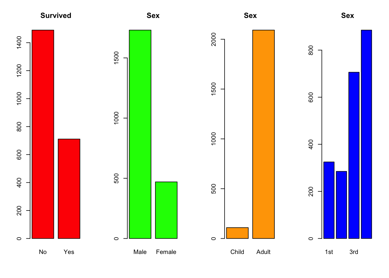 However, the way to answer our question will require thinking about more
than one variable at a time, and how they may (or may not) interact.
However, the way to answer our question will require thinking about more
than one variable at a time, and how they may (or may not) interact.
Let’s focus on the class of the passengers (Class) and
their survival (Survived). The class variable has 4
possible values (1st, 2nd, 3rd, Crew), and survival has 2 possibilities
(Yes,No) - thus we have 8 possible
combinations. We can summarise the counts of passengers in each
combination in a \(4\times2\) table. As
we are tabulating two variables, this is called a 2-way
contingency table:
library(knitr)
kable(xtabs(Freq~Survived+Class,data=titanic))| 1st | 2nd | 3rd | Crew | |
|---|---|---|---|---|
| No | 122 | 167 | 528 | 673 |
| Yes | 203 | 118 | 178 | 212 |
It can also be useful to append the totals for each row and column to the summary:
library(knitr)
tab <- xtabs(Freq~Survived+Class,data=titanic)
tab <- rbind(tab, apply(tab,2,sum))
tab <- cbind(tab, apply(tab,1,sum))
colnames(tab)[5] <- 'Total'
rownames(tab)[3] <- 'Total'
kable(tab)| 1st | 2nd | 3rd | Crew | Total | |
|---|---|---|---|---|---|
| No | 122 | 167 | 528 | 673 | 1490 |
| Yes | 203 | 118 | 178 | 212 | 711 |
| Total | 325 | 285 | 706 | 885 | 2201 |
Here we have summarised the fates of all the passengers, divided up by class or crew status. For example, we can easily see that far more 1st class passengers survived than did not, whereas the opposite was true for those in 3rd class. This would suggest that there is some association here to explore.
First, we need to set up a general 2-way contingency table problem. Suppose that:
- We have observed \(n\) individuals
- We have recorded that value of two categorical variables for each:
- Variable 1, which has \(C\) distinct levels
- Variable 2, which has \(R\) distinct levels
- The number of individuals who are observed in level \(i\) for variable 1 and level \(j\) for variable 2 is called \(o_{ij}\).
We can then summarise this in the 2-way table below, where the levels of variable 1 are the rows of the table, and the levels of variable 2 are the columns:
| Var 1\ Var 2 | 1 | 2 | … | \(j\) | … | \(C\) | Total |
|---|---|---|---|---|---|---|---|
| 1 | \(o_{11}\) | \(o_{12}\) | … | \(o_{1j}\) | … | \(o_{1C}\) | \(r_1\) |
| 2 | \(o_{21}\) | \(o_{22}\) | … | \(o_{2j}\) | … | \(o_{2C}\) | \(r_2\) |
| \(\vdots\) | \(\vdots\) | \(\vdots\) | \(\ddots\) | \(\vdots\) | \(\ddots\) | \(\vdots\) | \(\vdots\) |
| i | \(o_{i1}\) | \(o_{i2}\) | … | \(o_{ij}\) | … | \(o_{iC}\) | \(r_i\) |
| \(\vdots\) | \(\vdots\) | \(\vdots\) | \(\ddots\) | \(\vdots\) | \(\ddots\) | \(\vdots\) | \(\vdots\) |
| R | \(o_{R1}\) | \(o_{R2}\) | … | \(o_{Rj}\) | … | \(o_{RC}\) | \(r_R\) |
| Total | \(c_1\) | \(c_2\) | … | \(c_j\) | … | \(c_C\) | \(n\) |
Here we have also introduce notation for the row and columns sums:
- \(r_i\) is the sum of counts in the \(i\)th row. This corresponds to the number of observations of level \(i\) of Variable 1. The collection of row counts \(r_1,\dots,r_R\) corresponds to the counts for all the different levels of Variable 1.
- \(c_j\) is the sum of counts in the \(j\)th row. This corresponds to the number of observations of level \(j\) of Variable 2. The collection of row counts \(c_1,\dots,c_C\) corresponds to the counts for all the different levels of Variable 2.
1.3.1 Creating Contingency Tables
We can use the xtabs function from Lecture 1 to
construct these contingency tables from data. There are two different
usages, depending on whether the data has been pre-summarised as counts
(like the Titanic data), or if the data is not summarised and each row
corresponds to a single observation.
If the data is summarised already, and contains the totals in column
called counts, then the summary of counts for the levels of
variable1 is obtained by:
xtabs(counts~variable1, data=dataset)For example, to summarise survival:
xtabs(Freq~Survived,data=titanic)## Survived
## No Yes
## 1490 711For 2-way tables, we simply add another variable to the right of the
~ symbol:
xtabs(counts~variable1+variable2, data=dataset)For example, to summarise combinations of survival with class of passenger:
xtabs(Freq~Survived+Class,data=titanic)## Class
## Survived 1st 2nd 3rd Crew
## No 122 167 528 673
## Yes 203 118 178 212If the data contains one row per observation, then we have no
variable name to the left of the ~ symbol. For example, the
arthritis data contains information on the response to an
arthritis treatment. The data look like this:
load('arthritis.Rda')
head(arthritis[,c(2,3,5)])
## Treatment Sex Improved
## 1 Treated Male Some
## 2 Treated Male None
## 3 Treated Male None
## 4 Treated Male Marked
## 5 Treated Male Marked
## 6 Treated Male MarkedNote how each row just lists a combination of categories for the different variables, and we see many repetitions where different individuals have the same combinations.
To summarise the Treatment variable only, we would use the command
xtabs(~Treatment,data=arthritis)## Treatment
## Placebo Treated
## 43 41and the combinations of patient improvement with treatment:
xtabs(~Treatment+Improved,data=arthritis)## Improved
## Treatment None Some Marked
## Placebo 29 7 7
## Treated 13 7 211.3.2 n-way Contingency Tables
When we have \(n\) categorical variables, we could create an \(n\)-way contingency table. The table would summarise the counts of every possible combination of every possible level of the \(n\) variables. This obviously gets more complicated with larger \(n\), but we’ll come back to this later.
For instance, we could summarise the combinations of Titanic passenger survival, passenger class and passenger sex:
xtabs(Freq~Survived+Class+Sex, data=titanic)## , , Sex = Male
##
## Class
## Survived 1st 2nd 3rd Crew
## No 118 154 422 670
## Yes 62 25 88 192
##
## , , Sex = Female
##
## Class
## Survived 1st 2nd 3rd Crew
## No 4 13 106 3
## Yes 141 93 90 20Now we should have a 3-dimensional table with \(2\times 4\times 2\) cells! But R can only
print at most 2-dimensional tables. Instead, it has given us two
separate 2-way table for Survived+Class, one for each of
Sex=Male (top) and Sex=Female (bottom). We can
note here that Female passengers and crew had better survivale than
their male counterparts (with a notable exception being those in 3rd
class).
1.4 A Test for Contingency Tables
Exploring the independence of a pair of variables can lead to valuable insights in exploration and modelling. Specifically, we are interested in associations (or lack of associations) between variables, as these often point to potential interesting relationships in the data.
Typically, in statistics, we frame this problem from the opposite perspective and ask whether there is an absence of association or dependency between variables. This absence of association corresponds to the concept of independence of the corresponding variables, which is associated with statistical and probabilistic properties that can be investigated.
For example, we could ask whether Survived is
independent from Class in the Titanic data. If we find
evidence to the contrary, then we may conclude there is an association
or relationship between the two. The key idea behind using independence
as the property to verify is that if two variables \(X\) and \(Y\) are independent, then we can write
\[P[X=x,Y=y]=P[X=x]P[Y=y],\] or
equivalently in terms of conditional probabilitiy: \[P[X=x | Y=y]=P[X=x].\] The second version
tells us that even if I were to tell you the value of Y, that
would not cause you to change your probability distribution for \(X\). In other words, knowing \(Y\) has no influence on how we thinkg \(X\) will behave - in other words, the two
variables are completely unrelated.
We’ll develop a simple test for assessing this, based on these simple
equations. As a running example, let’s continue with the Titanic data
and investigate possible relationships between Survived and
Class. The idea behind our test is as follows:
- Using the data, we can estimate the probabilities of the different
levels of
Survived(\(p_i\)) andClass(\(p_j\)) separately using the proportions of the data observed in each category. - Under a hypothesis of independence, I can use the first equation
above to tell me that the probability of any combination of
SurvivedandClassis just the product of individual probabilities from the previous step, \(p_{ij}=p_i p_j\). Applying this to all combinations of categories gives me the probability for every possible combination of the two variables, \(p_{ij}\). - The expected number of observations in each combination of categories is obtained by multiplying the probabilities from step 2 by the sample size \(n\). This gives the expected counts for every combination, \(E_{ij}=np_{ij}\).
- We can then compare our expected counts to the observed counts in the data, and construct a test statistic.
Let’s see how this goes with our data:
Observed counts: We observe the following counts of the different categories ofSurvived and Class
| No | Yes |
|---|---|
| 1490 | 711 |
| 1st | 2nd | 3rd | Crew |
|---|---|---|---|
| 325 | 285 | 706 | 885 |
| No | Yes |
|---|---|
| 0.676965 | 0.323035 |
| 1st | 2nd | 3rd | Crew |
|---|---|---|---|
| 0.1476602 | 0.1294866 | 0.3207633 | 0.40209 |
Unsuprisingly, the more common categories are now associated with larger proportions.
Probabilities of combinations under independence We assume the null hypothesis to be \(H_0\): survival is independent from class. Then we can say, for example:
\[P[Survived=Yes,Class=1st] = P[Survived=Yes]\times P[Class=1st],\]
and the same for all the other combinations. By multiplying our probabilities from the previous step, we can make the following probability table for the joint distribution ofSurvived
and Class under our null hypothesis of independence:
| 1st | 2nd | 3rd | Crew | |
|---|---|---|---|---|
| No | 0.0999608 | 0.0876579 | 0.2171455 | 0.2722008 |
| Yes | 0.0476994 | 0.0418287 | 0.1036178 | 0.1298891 |
| 1st | 2nd | 3rd | Crew | |
|---|---|---|---|---|
| No | 220.0136 | 192.93503 | 477.9373 | 599.114 |
| Yes | 104.9864 | 92.06497 | 228.0627 | 285.886 |
We can now compare these expected counts with the ones we actually observed. If we find big differences, then we would conclude our hypothesis of independence must be wrong and that there is evidence of some form of relationship.
Before we do that, however, we’ll just set this up mathematically so we can obtain a formula for our test statistic.
1.4.1 The maths bit
Let \(O_{ij}\) be the observed count for the combination of category \(i\) of variable 1, and category \(j\) of variable 2. This comes from our data, and is in the \(i\)th row and \(j\)th column of our 2-way table.
We estimate the probability of observing category \(i\) of variable 1 as the proportion of the \(n\) observations which have category \(i\). From our 2-way table setup, this is the number of observations in row \(i\), denoted \(r_i\), divided by \(n\). Similarly, for variable 2 category \(j\) the proportion we seek is the number of observations in column \(j\), denoted \(c_j\), divided by \(n\). This gives us: \[P[\text{Variable 1}=i]=\frac{r_i}{n}, ~~~~ P[\text{Variable 2}=j]=\frac{c_j}{n},\] for \(i=1,\dots,R\), and \(j=1,\dots,C\).
Under the null hypothesis \(H_0\): variable 1 is independent from variable 2 and we can express the probability of the combination of Variable 1 category \(i\) with Variable 2 category \(j\) as:
\[\begin{align*} P[\text{Variable 1}=i ~\&~\text{Variable 2}=j] &=P[\text{Variable 1}=i]\times P[\text{Variable 2}=j]\\ &=\frac{r_i}{n}\times\frac{c_j}{n}\\ &=\frac{r_ic_j}{n^2}=p_{ij}. \end{align*}\]
If this is the probability of getting combination \((i,j)\), then out of \(n\) observations we would expect to see this combination \(n\times p_{ij}\) times: \[\begin{align*} E_{ij} &= np_{ij} = n\frac{r_ic_j}{n^2}\\ &=\frac{r_ic_j}{n}. \end{align*}\]
We call \(E_{ij}\) the expected count for the \(i,j\) combination of variable 1 and variable 2.
The \(\chi^2\) test statistic for this contingency table is then: \[X^2 = \sum_{i=1}^{R}\sum_{j=1}^C \frac{(O_{ij}-E_{ij})^2}{E_{ij}},\]
which gets compared to critical values from a \(\chi^2\) distribution with parameter (“degrees of freedom”) \(k=(R-1)\times(C-1)\).
We can expanded this idea to consider combinations of more than two variables using exactly the same calculations, but we’ll stop here!
1.5 Performing \(\chi^2\) tests
For the Titanic data problem, we can construct the test statistic using the method above and get a test statistic of \(X^2=190.46\) (check!). Comparing to the \(\chi^2\) distribution - this has a \(p\)-value of approximately 0! So, we strongly reject the hypothesis of independence and would do so at any of the usual levels of significance. Survival of the Titanic disaser and passenger class appear to be related!
Having discovered an interesting relationship, a good question to ask now is: why? Why did we reject this hypothesis? What about the data seemed to be at odds with the variables being independent?
To answer this, we look at the Pearson residuals - the components inside the double sum in our test statistic. For each combination of categories, we get a value of\(\frac{(O_{ij}-E_{ij})^2}{E_{ij}}\). We can inspect those values and see what we find. In particular, large values of the residuals indicate substantial departures from the null hypothesis. The sign of the residuals indicates whether there are \(\color{red}{\text{fewer}}\) (<0), or \(\color{red}{\text{more}}\) (>0) values than expected under independence.
| 1st | 2nd | 3rd | Crew | |
|---|---|---|---|---|
| No | \(\color{blue}{\text{-6.608}}\) | \(\color{blue}{\text{-1.867}}\) | \(\color{red}{\text{2.290}}\) | \(\color{red}{\text{3.019}}\) |
| Yes | \(\color{red}{\text{9.566}}\) | \(\color{red}{\text{2.703}}\) | \(\color{blue}{\text{-3.315}}\) | \(\color{blue}{\text{-4.370}}\) |
Here we notice the very large values in the 1st class column - we see far \(\color{red}{\text{more}}\) survivors than expected and far \(\color{red}{\text{fewer}}\) fatalities. The pattern appears to be reversed for those in 3rd class and the ship’s crew. Clearly, first class passengers had far better outcomes than would be expected if the chances were equal for everyone on board.
Finally, there’s no real need to do this entire calculation by hand
as R easily perform an independence test for a contingency table. All we
need to supply is the table of observed values obtained from
xtabs:
chisq.test( xtabs(Freq~Survived+Class,data=titanic) )##
## Pearson's Chi-squared test
##
## data: xtabs(Freq ~ Survived + Class, data = titanic)
## X-squared = 190.4, df = 3, p-value < 2.2e-162 Summary
- Categorical data should not be treated as quantitative, and care must be taken to ensure appropriate methods are used
- The \(\chi^2\) test provides a simple test of a categorical data table against a hypothesised distribution, or just a distribution which displays independence.
- This allows us to explore associations between categorical variables, which can be valuable for future exploration and modelling
- The
chisq.testfunction can take care of most of the calculation, though the reasoning behind the test is quite straightforward. - Inspecting the Pearson residuals can expose where the departures from the hypothesis occur.
2.1 Modelling and Testing
- Small tables - when working with \(\chi^2\) tests for small tables, it is recommended to apply a continuity correction to the test statistic Yates’ correction).
- Classification problems have categorical response variables. These methods will be useful to explore potential categorical predictors
- Categorical data models include loglinear models, logistic/multinomial regression, generalised linear models
- Patterns of association can be visualised using mosaic plots (see next lecture!)