Lab 1 - Introduction
Lab 1: Introduction
In this session, we are going to see how to effectively produce data
consisting of many features (variables) and how to perform some useful
computation with it. In exercise 1, we will look at an example of
multivariate data; in exercise 2, we will explore how we can measure the
distance between two observations; in exercises 3 and 4, we will learn
the commands that perform eigendecomposition and singular value
decomposition. This will be useful when performing Principal Component
Analysis.
Exercise 1 (Multivariate normal distribution)
We want to generate a data set with \(n\) observations and \(p\) features. The corresponding data matrix is the following \(n \times p\) matrix:
\(\mathbf{X} = \begin{pmatrix} x_{11} & x_{12} & \cdots & x_{1p} \\ x_{21} & x_{22} & \cdots & x_{2p} \\ \vdots & \vdots & \vdots & \vdots\\ x_{n1} & x_{n2} & \cdots & x_{np} \\ \end{pmatrix}\).
Read more
Multivariate, in this situation, means that \(p > 2\). When \(p=1\) the data set is called univariate, when \(p=2\) it is called bivariate.A common way to generate data is using probability distributions. For this exercise, we will make a popular choice and use the multivariate standard normal distribution (aka multivariate Gaussian distribution) \(N(\boldsymbol{\mu} = \boldsymbol{0}, \boldsymbol{\Sigma}=\boldsymbol{I})\). This is the unique
Read more
Multivariate normal distributions are the most studied and most useful of multivariate probability distributions. A vector of random variables \(\mathbf{X}:= \begin{pmatrix} X_1\\ \vdots\\ X_n \end{pmatrix}\) is said to be normally distributed if every linear combination \(a_1 X_1 + \dots + a_n X_n\) is normally distributed.
The multivariate Gaussian distribution \(N(\boldsymbol{\mu} = \boldsymbol{0}, \boldsymbol{\Sigma}=\boldsymbol{I})\) is the special case of a multivariate normal that has mean \(\boldsymbol{0}\) (the vector whose elements are all zero) and covariance matrix \(\boldsymbol{I}\) (the identity matrix of dimension \(p \times p\)).With this theoretical framework in mind, let us simulate some data:
-
Load the following package into your workspace.
library(MASS) -
run ?mvrnorm in console and see Help tab to check how to use this function to generate data from a multivariate normal distribution.
?mvrnorm
You are now ready to perform the following tasks:
Task 1a
Generate the multivariate Gaussian data \(\mathbf{X} \sim N(\boldsymbol{0},
\mathbf{I}_p)\) with \(n=50\)
and \(p=10\), and check its
dimension.
Click for solution
n <- 50
p <- 10
mu <- rep(0, p)
Sigma <- diag(p)

set.seed(2024)
dat <- mvrnorm(n = n, mu = mu, Sigma = Sigma)
dim(dat)
## [1] 50 10
Task 1b
Obtain the estimated mean vector \(\hat{\mu}\) and check it is close to the
true parameters, \(\mu\).
Click for solution
muhat <- colMeans(dat)
cbind(mu, muhat)
## mu muhat
## [1,] 0 0.02471851
## [2,] 0 0.12684999
## [3,] 0 0.05368035
## [4,] 0 0.05309381
## [5,] 0 0.05201272
## [6,] 0 0.10833111
## [7,] 0 0.23795856
## [8,] 0 0.02617100
## [9,] 0 -0.09426008
## [10,] 0 -0.07560478
Task 1c
Compute the estimated covariance matrix \(\hat{\Sigma}\) and check that it is close
to the true covariance matrix \(\Sigma\). Comparing large matrices by eyes
is a bit tricky. Can you think of a better way to visually do this
comparison?
Click for solution
Sigmahat <- cov(dat)
par(mfrow=c(1, 2))
image(Sigma, main = "True covariance", axes=FALSE)
image(Sigmahat, main = "Estimated covariance", axes=FALSE)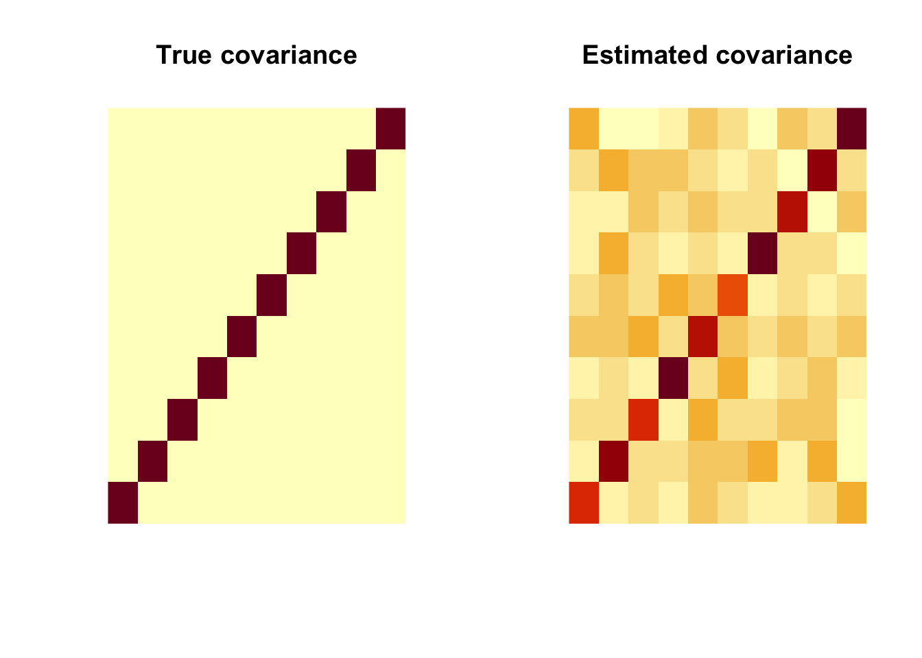
That’s not quite what we expected. Why? because image() in R rotates the matrix. So we need to change the input.
par(mfrow=c(1, 2))
image(Sigma[,nrow(Sigma):1], main = "True covariance", axes=FALSE)
image(Sigmahat[,nrow(Sigmahat):1], main = "Estimated covariance", axes=FALSE)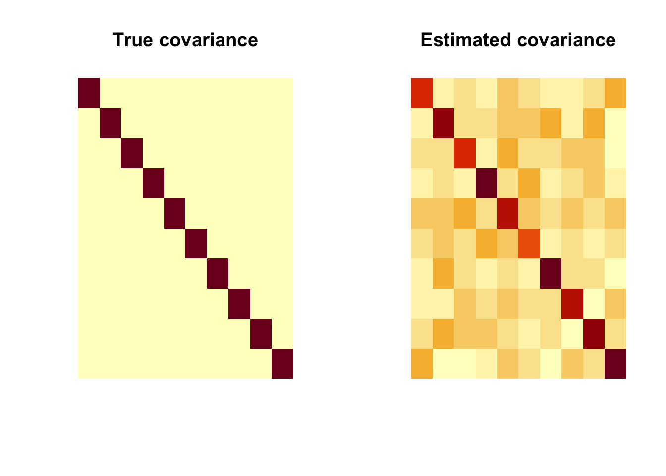
Exercise 2 (Distance measure)
Let us now compute the distance between data points, starting with a
bivariate case (\(p=2\)) and ending
with a multivariate example (\(p=10\)).
Task 2a
Simulate the bivariate Gaussian data \(\mathbf{X} \sim N(\boldsymbol{0},
\mathbf{I}_p)\) with \(n=2\) and
\(p=2\), and point two observations in
a coordinate plan (plotting dots) using different colours. Let the first
variable corresponds to \(x\) axis and
the second variable corresponds to \(y\) axis. (If you have no idea how to add a
dot in a plot, run ?points in console to get a hint.)
Click for solution
n <- 2
p <- 2
mu <- rep(0, p)
Sigma <- diag(p)

set.seed(2024)
dat <- mvrnorm(n = n, mu = mu, Sigma = Sigma)
obs1 <- dat[1,]
obs2 <- dat[2,]

plot(obs1[1], obs1[2], type="p", xlab="x", ylab="y", xlim=range(dat[,1]), ylim=range(dat[,2]))
points(obs2[1], obs2[2], col=2)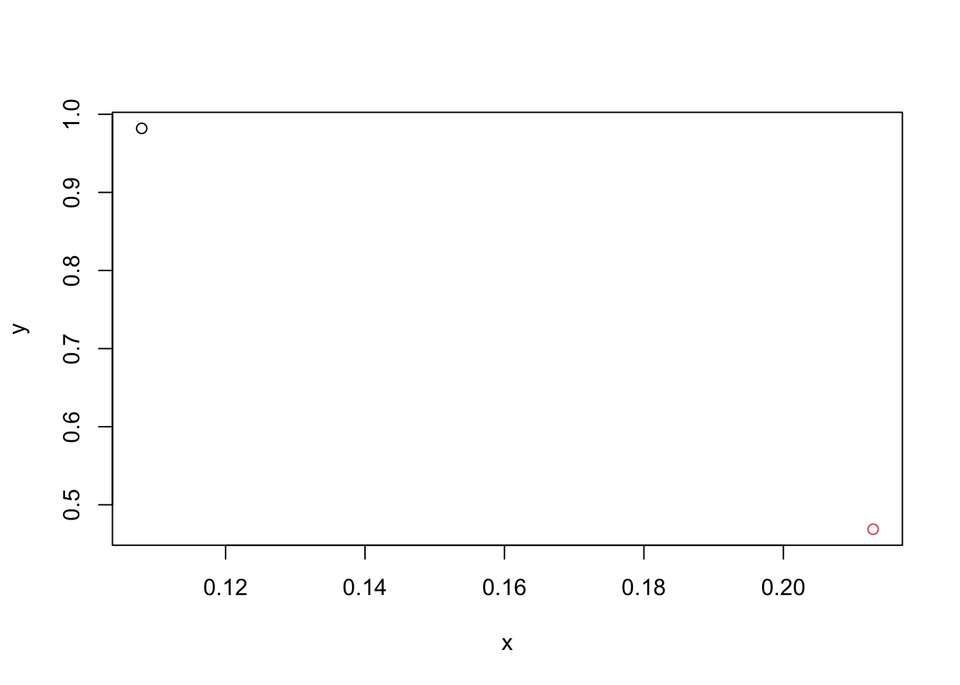
Task 2b
Plot the shortest path between these two dots and compute its length.
This is the Euclidean distance between your data
points. (running ?segments would be helpful.)
Click for solution
plot(obs1[1], obs1[2], type="p", xlab="x", ylab="y", xlim=range(dat[,1]), ylim=range(dat[,2]))
points(obs2[1], obs2[2], col=2)
segments(x0=obs1[1], y0=obs1[2], x1=obs2[1], y1=obs2[2], col=4, lty=2)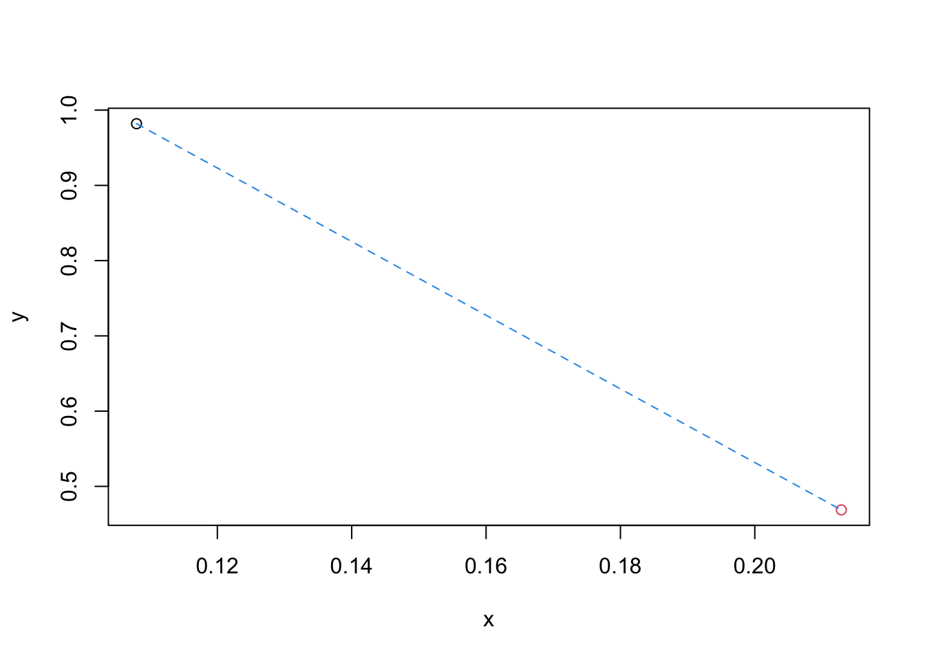
# 1) calculating by hand using the formula
d <- sqrt((obs2[1]-obs1[1])^2 + (obs2[2]-obs1[2])^2)
d
## [1] 0.5238659# 2) using the "norm" function in R
norm(obs1-obs2, type="2")## [1] 0.5238659
Task 2c
Now, we will do the same for p greater than 2. Generate the
multivariate Gaussian data \(\mathbf{X} \sim
N(\boldsymbol{0}, \mathbf{I}_p)\) with \(n=2\) and \(p=10\), and find the Euclidean distance
between these two data points.
Click for solution
n <- 2
p <- 10
mu <- rep(0, p)
Sigma <- diag(p)

set.seed(2024)
dat <- mvrnorm(n = n, mu = mu, Sigma = Sigma)
obs1 <- dat[1,]
obs2 <- dat[2,]

# 1) calculating by hand using the formula
d <- sqrt(sum((obs2-obs1)^2))
d
## [1] 4.179483# 2) using the "norm" function in R
norm(obs1-obs2, type="2")## [1] 4.179483
Exercise 3 (Eigendecomposition)
The covariance matrix of a multivariate data set is symmetric, so it can be decomposed as above. Let us check this on the covariance matrix of \(X\) where \(\mathbf{X} \sim N(\boldsymbol{0}, \mathbf{I}_p)\) with \(n=100\) and \(p=3\).
n <- 100
p <- 3
mu <- rep(0, p)

set.seed(2024)
X <- mvrnorm(n = n, mu = mu, Sigma = diag(p))
Sigmahat <- cov(X)
Task 3a
Perform the eigendecomposition of the estimated covariance matrix using eigen() function in R. Run ?eigen to see how to use the function. Find the matrices \(P\) and \(\Lambda\) from the results.
Click for solution
eigdec <- eigen(Sigmahat)
eigdec
## eigen() decomposition
## $values
## [1] 1.1199814 0.9914944 0.7753919
##
## $vectors
##            [,1]       [,2]        [,3]
## [1,]  0.2071519 -0.1921031  0.95926248
## [2,] -0.6349900 -0.7723212 -0.01754045
## [3,] -0.7442283 0.6054885 0.28197133Lambda <- diag(eigdec$values)
Lambda## [,1] [,2] [,3]
## [1,] 1.119981 0.0000000 0.0000000
## [2,] 0.000000 0.9914944 0.0000000
## [3,] 0.000000 0.0000000 0.7753919P <- eigdec$vectors
P## [,1] [,2] [,3]
## [1,] 0.2071519 -0.1921031 0.95926248
## [2,] -0.6349900 -0.7723212 -0.01754045
## [3,] -0.7442283 0.6054885 0.28197133
Task 3b
Check that \(\hat{\Sigma} = P \Lambda P^t\) as the maths predict.
Click for solution
Sigmahat## [,1] [,2] [,3]
## [1,] 0.79815382 -0.01326497 -0.07826101
## [2,] -0.01326497 1.04323544 0.06178886
## [3,] -0.07826101 0.06178886 1.04547838P%*%Lambda%*%t(P)## [,1] [,2] [,3]
## [1,] 0.79815382 -0.01326497 -0.07826101
## [2,] -0.01326497 1.04323544 0.06178886
## [3,] -0.07826101 0.06178886 1.04547838Task 3c
Find the eigenvalues of the inverse matrix of \(\hat{\Sigma}\). Compare it with the eigenvalues of \(\hat{\Sigma}\). What is their relationship?
Click for solution
e1 = eigen(Sigmahat)$values

e2 = eigen(solve(Sigmahat))$values

e2
## [1] 1.289670 1.008579 0.892872sort(1/e1, decreasing = T)## [1] 1.289670 1.008579 0.892872
Exercise 4 (Singular Value Decomposition)
Our test matrix for the singular value decomposition will be the data matrix \(\mathbf{X}\) (we then assume to have \(n>p\)).
Task 4a
Perform the singular value decomposition of the data matrix \(\mathbf{X}\) using the svd()
function in R.
To do this, first centre the matrix \(X\) using the R command scale so
that the mean of our sample is exactly 0. Then, find the matrices \(U\), \(D\)
and \(V\) as above and check that \(X = UDV^t\).
These matrices are too big to be compared by eyes. What would be a
reasonable way to perform this check?
Click for solution
X1 <- scale(X)
svdec <- svd(X1)

U <- svdec$u
V <- svdec$v
D <- diag(svdec$d)

range(X1-U%*%D%*%t(V))
## [1] -3.552714e-15 3.108624e-15
Task 4b
Check that the matrices \(U\) and \(V\) both have orthonormal columns.Hint:
it is enough to verify that \(U^t U = V^t V = \mathbf{I}\).
Click for solution
# Method 1: using the 'range' function
range(t(U)%*%U-diag(p))
## [1] -4.440892e-16 2.012279e-16range(t(V)%*%V-diag(p) )## [1] -6.661338e-16 0.000000e+00# Method 2: using the 'round' function
round(t(U)%*%U, 10)## [,1] [,2] [,3]
## [1,] 1 0 0
## [2,] 0 1 0
## [3,] 0 0 1round(t(V)%*%V, 10)## [,1] [,2] [,3]
## [1,] 1 0 0
## [2,] 0 1 0
## [3,] 0 0 1
Task 4c
Compare the matrix \(D\) with the matrix \(\Lambda\) obtained in Exercise 3. What is their relationship and why?
Hint:
Compare \(D/\sqrt{n-1}\) and \(\sqrt{\Lambda}\), the matrix obtained by applying the square root transformation to all elements of \(\Lambda\).
Click for solution
eigdec <- eigen(cov(X1))
Lambda <- diag(eigdec$values)

sqrt(Lambda)
## [,1] [,2] [,3]
## [1,] 1.054158 0.0000000 0.0000000
## [2,] 0.000000 0.9931967 0.0000000
## [3,] 0.000000 0.0000000 0.9499007D/sqrt(n-1)## [,1] [,2] [,3]
## [1,] 1.054158 0.0000000 0.0000000
## [2,] 0.000000 0.9931967 0.0000000
## [3,] 0.000000 0.0000000 0.9499007Why are the results the same? Remember that we scaled \(\mathbf{X}\) in such a way that the mean of its columns is \(\mathbf{0}\). Hence, the estimated covariance matrix is \(\hat{\Sigma}=\frac{1}{n-1} X X^t\). Hence, the eigenvalues of \(X X^t\) are \(n-1\) times those of \(\hat{\Sigma}\), namely the elements on the diagonal of \(\Lambda\).
On the other hand, singular value decomposition gives us \[\begin{align*} &X^t X = V D^t U^t UD V^t = V D^2 V^t, \end{align*}\] so the eigenvalues of \(X X^t\) are also the squares of the elements on the diagonal of \(D\)!
Upshot: we have two methods to compute these eigenvalues (eigendecomposition and singular value decomposition). We will use this when doing Principal Component Analysis.