Chapter 4 Supervised Learning — Regression
4.1 Historical notes
Regression is an important technique in statistics and machine learning. It was first introduced by Sir Francis Galton in the 19th century. He used it to study the relationship between the heights of fathers and their sons. The term “regression” was coined by Galton to describe the tendency of the heights of sons to “regress” towards the mean height of the population. For us, the general idea is to predict a continuous value from a set of input variables.
As we have already seen, metrics for regression are different from those for classification. Historically, machine learning techniques for regression have focused on getting as close as possible to the target variable with little regard for prediction uncertainty. This is changing as we move towards more complex models that can provide a measure of uncertainty in their predictions.
4.2 Running example
Like in the previous chapter, we will use two well known data sets to illustrate regression techniques. The first is the Boston housing data set, which contains information about housing in the Boston area. The target variable is the median value of owner-occupied homes in thousands of dollars. The data set contains 506 observations on 14 variables. The second data set is the Auto MPG data set, which contains information about cars. The target variable is the miles per gallon (MPG) of the car. The data set contains 398 observations on 9 variables.
In both cases, it is trivial to set up a linear regression model in R.
# load in the data
library(MASS)
data(Boston)
data(mtcars)

# standardise the data to aid interpretation
Boston <- as.data.frame(scale(Boston))
mtcars <- as.data.frame(scale(mtcars))

# linear regression
lm.fit.Boston <- lm(medv ~ ., data = Boston)
summary(lm.fit.Boston)
##
## Call:
## lm(formula = medv ~ ., data = Boston)
##
## Residuals:
## Min 1Q Median 3Q Max
## -1.69559 -0.29680 -0.05633 0.19322 2.84864
##
## Coefficients:
## Estimate Std. Error t value Pr(>|t|)
## (Intercept) -1.628e-16 2.294e-02 0.000 1.000000
## crim -1.010e-01 3.074e-02 -3.287 0.001087 **
## zn 1.177e-01 3.481e-02 3.382 0.000778 ***
## indus 1.534e-02 4.587e-02 0.334 0.738288
## chas 7.420e-02 2.379e-02 3.118 0.001925 **
## nox -2.238e-01 4.813e-02 -4.651 4.25e-06 ***
## rm 2.911e-01 3.193e-02 9.116 < 2e-16 ***
## age 2.119e-03 4.043e-02 0.052 0.958229
## dis -3.378e-01 4.567e-02 -7.398 6.01e-13 ***
## rad 2.897e-01 6.281e-02 4.613 5.07e-06 ***
## tax -2.260e-01 6.891e-02 -3.280 0.001112 **
## ptratio -2.243e-01 3.080e-02 -7.283 1.31e-12 ***
## black 9.243e-02 2.666e-02 3.467 0.000573 ***
## lstat -4.074e-01 3.938e-02 -10.347 < 2e-16 ***
## ---
## Signif. codes: 0 '***' 0.001 '**' 0.01 '*' 0.05 '.' 0.1 ' ' 1
##
## Residual standard error: 0.516 on 492 degrees of freedom
## Multiple R-squared: 0.7406, Adjusted R-squared: 0.7338
## F-statistic: 108.1 on 13 and 492 DF, p-value: < 2.2e-16##
## Call:
## lm(formula = mpg ~ ., data = mtcars)
##
## Residuals:
## Min 1Q Median 3Q Max
## -0.57254 -0.26620 -0.01985 0.20230 0.76773
##
## Coefficients:
## Estimate Std. Error t value Pr(>|t|)
## (Intercept) -1.613e-17 7.773e-02 0.000 1.0000
## cyl -3.302e-02 3.097e-01 -0.107 0.9161
## disp 2.742e-01 3.672e-01 0.747 0.4635
## hp -2.444e-01 2.476e-01 -0.987 0.3350
## drat 6.983e-02 1.451e-01 0.481 0.6353
## wt -6.032e-01 3.076e-01 -1.961 0.0633 .
## qsec 2.434e-01 2.167e-01 1.123 0.2739
## vs 2.657e-02 1.760e-01 0.151 0.8814
## am 2.087e-01 1.703e-01 1.225 0.2340
## gear 8.023e-02 1.828e-01 0.439 0.6652
## carb -5.344e-02 2.221e-01 -0.241 0.8122
## ---
## Signif. codes: 0 '***' 0.001 '**' 0.01 '*' 0.05 '.' 0.1 ' ' 1
##
## Residual standard error: 0.4397 on 21 degrees of freedom
## Multiple R-squared: 0.869, Adjusted R-squared: 0.8066
## F-statistic: 13.93 on 10 and 21 DF, p-value: 3.793e-07The summaries here give us the adjusted R-squared amongst other things. It is interesting to consider the model coefficients in these models and to look at which are significantly different from zero. We can also calculate the other performance measures that we met in the earlier chapter using the fitted models.
| Boston | Auto MPG | |
|---|---|---|
| MSE | 0.26 | 0.13 |
| RMSE | 0.51 | 0.36 |
| MAE | 0.36 | 0.29 |
| MSLE | NaN | NaN |
| MAPE | 2.51 | 0.64 |
You will note that some of these return NaN values. This is because the target variable contains zeros. We can remove these from the data set to avoid this issue or think more carefully about which metric is appropriate for the problem at hand. You will also note that in isolation these metrics are not particularly informative. They are useful for comparing models, but not for understanding the quality of the model.
4.3 Regularised regression
As already mentioned in the section on overfitting, regularisation is a technique that can be used to prevent overfitting. Regularisation adds a penalty term to the loss function that is minimised by the model. The penalty term is a function of the model parameters and is designed to prevent the model from becoming too complex. There are two common types of regularisation: L1 and L2. L1 regularisation is also known as Lasso regression, while L2 regularisation is known as Ridge regression. Elastic Net regression is a combination of L1 and L2 regularisation.
Recall that simple linear regression models are fitted by minimising the mean squared error (MSE) loss function. We find the coefficients for the linear model by minimising the following loss function:
\[ \text{Loss} = \sum_{i=1}^{n} (y_i - \widehat{y}_i)^2 \]
where \(y_i\) are the observed values, \(\widehat{y}_i\) are the predicted values, and \(n\) is the number of observations. The coefficients are found by minimising the loss function with respect to the model parameters. Let’s remind ourselves of the the coefficient estimate using least-squares:
\[ \widehat{\beta} = (X^T X)^{-1} X^T y \]
where \(X\) is the design matrix and \(y\) is the response variable. The design matrix is a matrix of the input variables with an additional column of ones for the intercept term. The coefficients are found by inverting the product of the transpose of the design matrix and the design matrix and multiplying the result by the transpose of the design matrix and the target variable.
When using regularised regression techniques, it is common to standardise both the explanatory variables and the response variable. This is because the regularisation terms are sensitive to the scale of the variables. Standardising the variables means that the regularisation terms are applied equally to all the variables.
4.3.1 Lasso regression
Lasso (Least Absolute Shrinkage and Selection Operator) regression adds a penalty term to the loss function that is the sum of the absolute values of the model parameters. The penalty term is multiplied by a hyperparameter \(\lambda\) that controls the strength of the regularisation. The loss function for Lasso regression is given by
\[ \begin{aligned} \text{Loss} &= \sum_{i=1}^{n} (y_i - \widehat{y}_i)^2 + \lambda \sum_{j=1}^{p} |\beta_j|\\ &= ||y - X\beta||_2^2 + \lambda ||\beta||_1 \end{aligned} \]
where \(\beta_i\) are the model parameters. Lasso regression is also called L1 regularisation because the penalty term is the L1 norm of the model parameters. The lasso regression model is trained by minimising this loss function, and we can find that the solution to the lasso regression problem is
\[ \widehat{\beta} = \text{argmin}_{\beta} \left( ||y - X\beta||_2^2 + \lambda ||\beta||_1 \right) \]
The powerful aspect of Lasso regression is that it can be used for variable selection. The L1 penalty term encourages sparsity in the model parameters, which means that some of the model parameters will be set to zero. This can be useful when there are many input variables and we want to identify the most important variables. From a Bayesian perspective, Lasso regression can be seen as a Bayesian model with a Laplace prior on the model parameters.
The minimisation of the loss function for Lasso regression can be solved using the coordinate descent algorithm. The coordinate descent algorithm works by iteratively updating the model parameters by minimising the loss function with respect to one model parameter at a time. The algorithm is guaranteed to converge to the optimal solution, but it may take a long time to converge.
At this point, it is worth noting that we should standardise both the explanatory variables and the response variable when using regularised regression techniques. This is because the regularisation terms are sensitive to the scale of the variables: standardising the variables means that the regularisation terms are applied equally to all the variables.
4.3.2 Ridge regression
Ridge regression adds a penalty term to the loss function that is the sum of the squares of the model parameters. The penalty term is again multiplied by a hyperparameter \(\lambda\) that controls the strength of the regularisation. The loss function for Ridge regression is given by
\[ \begin{aligned} \text{Loss} &= \sum_{i=1}^{n} (y_i - \widehat{y}_i)^2 + \lambda \sum_{j=1}^{p} \beta_j^2\\ &= ||y - X\beta||_2^2 + \lambda ||\beta||_2^2 \end{aligned} \]
where \(\beta_i\) are the model parameters. The Ridge regression model is trained by minimising this loss function and is also termed L2 regularisation because the penalty term is the L2 norm of the model parameters. With some rearrangement and using the design matrix notation, we can write the solution to the ridge regression problem as
\[ \widehat{\beta} = \left(X^{T} X + \lambda I\right)^{-1} X^{T} y. \]
We can see that this is a similar solution to the simple linear regression model, but with an additional term \(\lambda I\) in the inverse of the product of the transpose of the design matrix and the design matrix. From a Bayesian perspective, ridge regression can be seen as a Bayesian linear regression model with a Gaussian prior on the model parameters.
Figures 4.1 and 4.2 give the surfaces for loss functions under simple linear regression and for the ridge variant respectively. We can see that the shape of the contours is the same for both, but they are slightly steeper for the ridge variant and the minimum is closer to the origin. This is because the extra term in the loss function adds more information and makes us more sure about the estimates whilst also shrinking them towards zero.
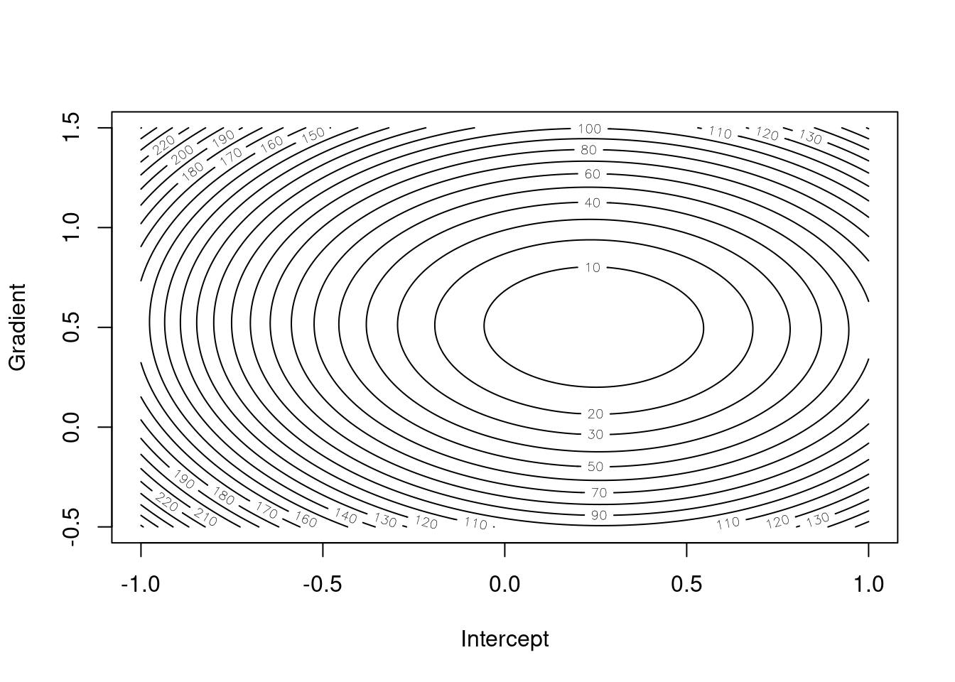
Figure 4.1: Simple linear regression loss function for different gradient/intercept pairs
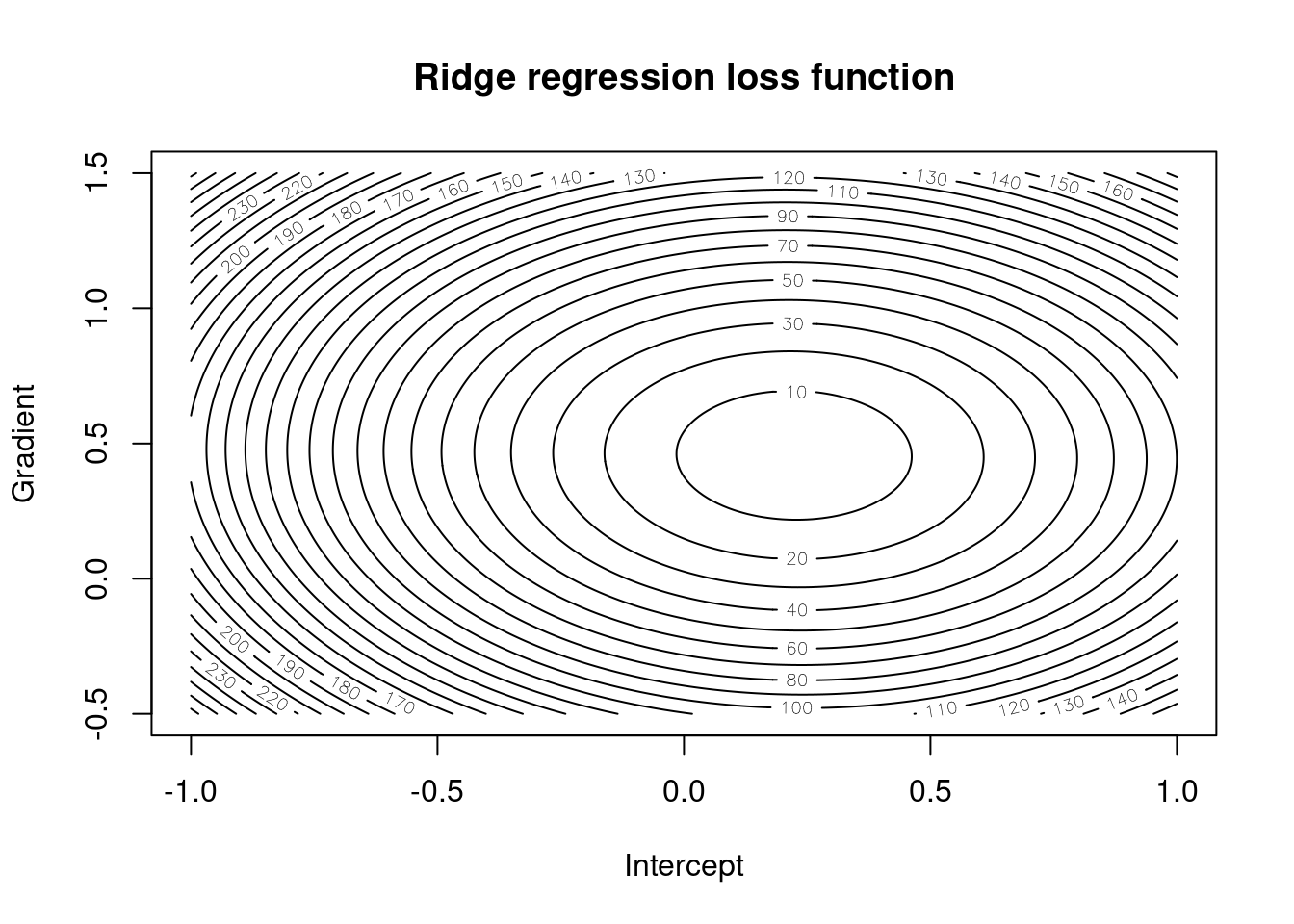
Figure 4.2: Ridge regression loss function
4.3.3 Elastic Net regression
Elastic Net regression is a combination of L1 and L2 regularisation. The loss function for Elastic Net regression is given by
\[ \begin{aligned} \text{Loss} &= \sum_{i=1}^{n} (y_i - \widehat{y}_i)^2 + \lambda \left( \alpha \sum_{j=1}^{p} |\beta_j| + (1-\alpha) \sum_{j=1}^{p} \beta_j^2 \right)\\ &= ||y - X\beta||_2^2 + \lambda \left( \alpha ||\beta||_1 + (1-\alpha) ||\beta||_2^2 \right) \end{aligned} \]
where \(\beta_i\) are the model parameters and \(\alpha\) and \(\lambda\) are hyperparameters that control the strength of the regularisation. The Elastic Net regression model is trained by minimising this loss function. Again, we can consider the Bayesian interpretation of Elastic Net regression as a Bayesian linear regression model with a mixture of Gaussian and Laplace priors on the model parameters.
4.3.4 Setting the hyperparameters
The hyperparameters in the penalty terms control the strength of the regularisation in Lasso, Ridge, and Elastic Net regression. There are two common techniques for selecting the hyperparameters: cross-validation and grid search. With cross-validation, the hyperparameters are chosen to minimise the loss function on a validation set. The hyperparameters can also be set using grid search. The hyperparameters are chosen by trying all possible combinations of values and selecting the combination that minimises the loss function on a validation set.
Example
First, we consider lasso and ridge regression for the Boston data set. Recall that the original linear regression model had an adjusted R-squared of 0.73 and an RMSE of 0.51. Also, the coefficients of the linear terms were:
##              [,1]
## (Intercept)  0.00
## crim        -0.10
## zn           0.12
## indus        0.02
## chas         0.07
## nox         -0.22
## rm           0.29
## age          0.00
## dis         -0.34
## rad          0.29
## tax         -0.23
## ptratio     -0.22
## black        0.09
## lstat       -0.41
Now, we fit a lasso regression model to the data set utilising the caret and elasticnet packages. The package elasticnet is used to fit the model, while caret is used to perform cross-validation.
library(caret)
set.seed(123)
tune_grid <- expand.grid(alpha = 1,
                         lambda = seq(0.01, 1,
                                      by = 0.01))
lasso.fit.Boston <- train(medv ~ .,
                          data = Boston,
                          method = "glmnet",
                          trControl = trainControl(method = "cv",
                                                   number = 10),
                          tuneGrid = tune_grid)
The lasso regression model has a RMSE of 1.
The coefficients of the linear terms are:
## 14 x 1 sparse Matrix of class "dgCMatrix"
##                s1
## (Intercept)  0.00
## crim        -0.07
## zn           0.08
## indus        .
## chas         0.07
## nox         -0.18
## rm           0.31
## age          .
## dis         -0.27
## rad          0.14
## tax         -0.10
## ptratio     -0.21
## black        0.08
## lstat       -0.41
We see that two of the variables are ignored by the lasso regression model. For the remaining 12 coefficients, they have been pulled towards zero.
4.4 \(k\)-nearest neighbours
Like in the classification setting, we can use \(k\)-nearest neighbours for regression. The idea is the exactly the same: we predict the target variable by averaging the values of the \(k\)-nearest neighbours. The updated algorithm is given by
- Calculate the distance between the test point and all the training points.
- Sort the distances and determine the \(k\)-nearest neighbours.
- Average the target variable of the \(k\)-nearest neighbours.
Again, the choice of \(k\) is important in \(k\)-nearest neighbours. A small value of \(k\) will result in a model that is sensitive to noise, while a large value of \(k\) will result in a model that is biased. The choice of \(k\) will depend on the problem at hand and the amount of noise in the data. More formally, the mathematical representation of the \(k\)-nearest neighbours algorithm is \[ \widehat{y} = \frac{1}{k} \sum_{i=1}^{k} y_i \] where \(\widehat{y}\) is the predicted value, \(k\) is the number of neighbours, and \(y_i\) is the target variable of the \(i\)-th neighbour.
Step 2 of the algorithm can be computationally challenging with large training sets. The knn package in R uses a data structure called a k-d tree to speed up the calculation of the distances between the test point and the training points. The \(k\)-d tree is a binary tree that is used to partition the input space into regions. The \(k\)-d tree is built by recursively splitting the input space along the dimensions of the input variables. The \(k\)-d tree is used to find the \(k\)-nearest neighbours by traversing the tree and only considering the regions that contain the \(k\)-nearest neighbours.
The final predictions can be thought of as a piecewise constant function over the input space defined by the training data. The different prediction values sit on a Voronoi tessellation whose tiles are determined by the training data. The idea behind \(k\)-nearest neighbours is related to the idea of stacking that we will meet in the next section. Stacking uses the predictions of multiple models to make a final prediction. In the case of \(k\)-nearest neighbours, the prediction “models” are the \(k\)-nearest neighbours themselves.
Example
We fit a \(k\)-nearest neighbours model to the Boston data set using the knn package within caret.
set.seed(123)
# Set up train and test sets
trainIndex <- sample(1:nrow(Boston), 0.8 * nrow(Boston))
trainBoston <- Boston[trainIndex,]
testBoston <- Boston[-trainIndex,]

# Fit the model
knn.fit.Boston <- train(medv ~ .,
                        data = Boston,
                        method = "knn",
                        trControl = trainControl(method = "cv",
                                                 number = 10))

# Predictions
knn.pred <- predict(knn.fit.Boston, testBoston)
Figure 4.3 shows the model performance in terms of the actual and predicted values.
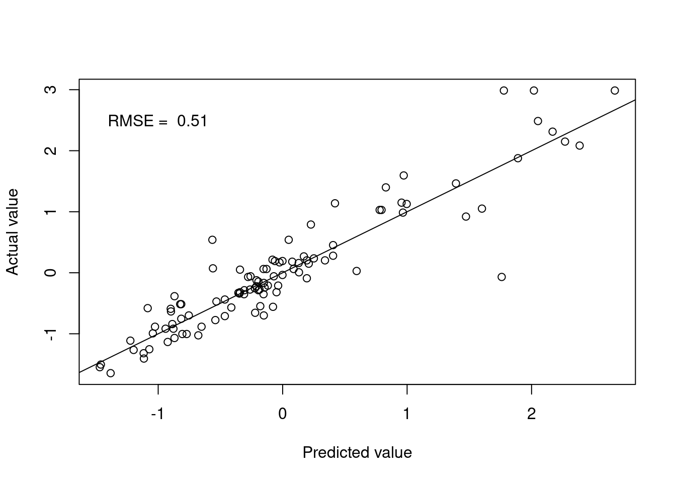
Figure 4.3: k-nearest neighbours predictions
We can extend the \(k\)-nearest neighbours model to include a weighting term in the prediction. The weighting term is a function of the distance between the test point and the training points. The idea is to give more weight to the training points that are closer to the test point. The weighted \(k\)-nearest prediction is calculated using
\[
\widehat{y} = \frac{\sum_{i=1}^{k} w_i y_i}{\sum_{i=1}^{k} w_i}
\]
where \(w_i\) is the weight of the \(i\)-th neighbour. The weights are typically calculated using the inverse of the distance between the test point and the training points. The weighted \(k\)-nearest neighbours model is implemented in the kknn package in R.
set.seed(123)
# Fit the model
kknn.fit.Boston <- train(medv ~ .,
                        data = Boston,
                        method = "kknn",
                        trControl = trainControl(method = "cv",
                                                 number = 10))

# Predictions
kknn.pred <- predict(kknn.fit.Boston, testBoston)
Figure 4.4 shows the model performance in terms of the actual and predicted values utilising the distance weights.
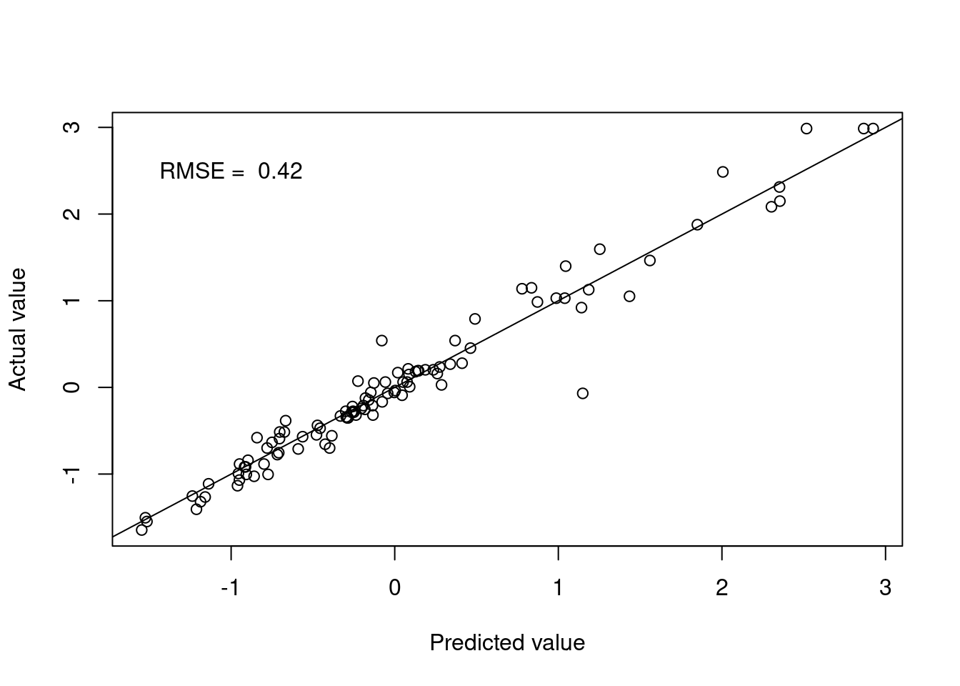
Figure 4.4: Weighted k-nearest neighbours predictions
4.5 Decision trees
Decision trees provide yet another non-parametric regression technique that is based on recursive partitioning of the input space that work the same way as in the classification setting. The idea is to split the input space into regions and fit a simple model to each region. The model is trained by recursively splitting the input space into regions until a stopping criterion is met. The stopping criterion can be based on the number of observations in a region, the depth of the tree, or the impurity of the regions. The impurity of a region is a measure of how well the target variable is predicted by the model in that region. The impurity can be measured using the mean squared error, the mean absolute error, or the mean squared logarithmic error.
In the standard implementation, the model is simply the mean of the target variable in the region. The final model is therefore a multidimensional step function over the space of explanatory variables.
Example
Let’s see it in action for the mtcars data set.
set.seed(123)
# Set up train and test sets
trainIndex <- createDataPartition(mtcars$mpg, p = 0.8,
                                  list = FALSE)
trainMtcars <- mtcars[trainIndex,]
testMtcars <- mtcars[-trainIndex,]

# Fit the model
tree.fit.mtcars <- train(mpg ~ .,
                         data = mtcars,
                         method = "rpart",
                         trControl = trainControl(method = "cv",
                                                  number = 10))

# Predictions
tree.pred <- predict(tree.fit.mtcars,
                     testMtcars)
Figures 4.5 and 4.6 show the model performance in terms of the actual and predicted values and the fitted decision tree. The model here is extremely simple with only two splits. Essentially, the model provides just three values for the mean behaviour of the target variable. This is to be expected given the small number of observations in the data set.
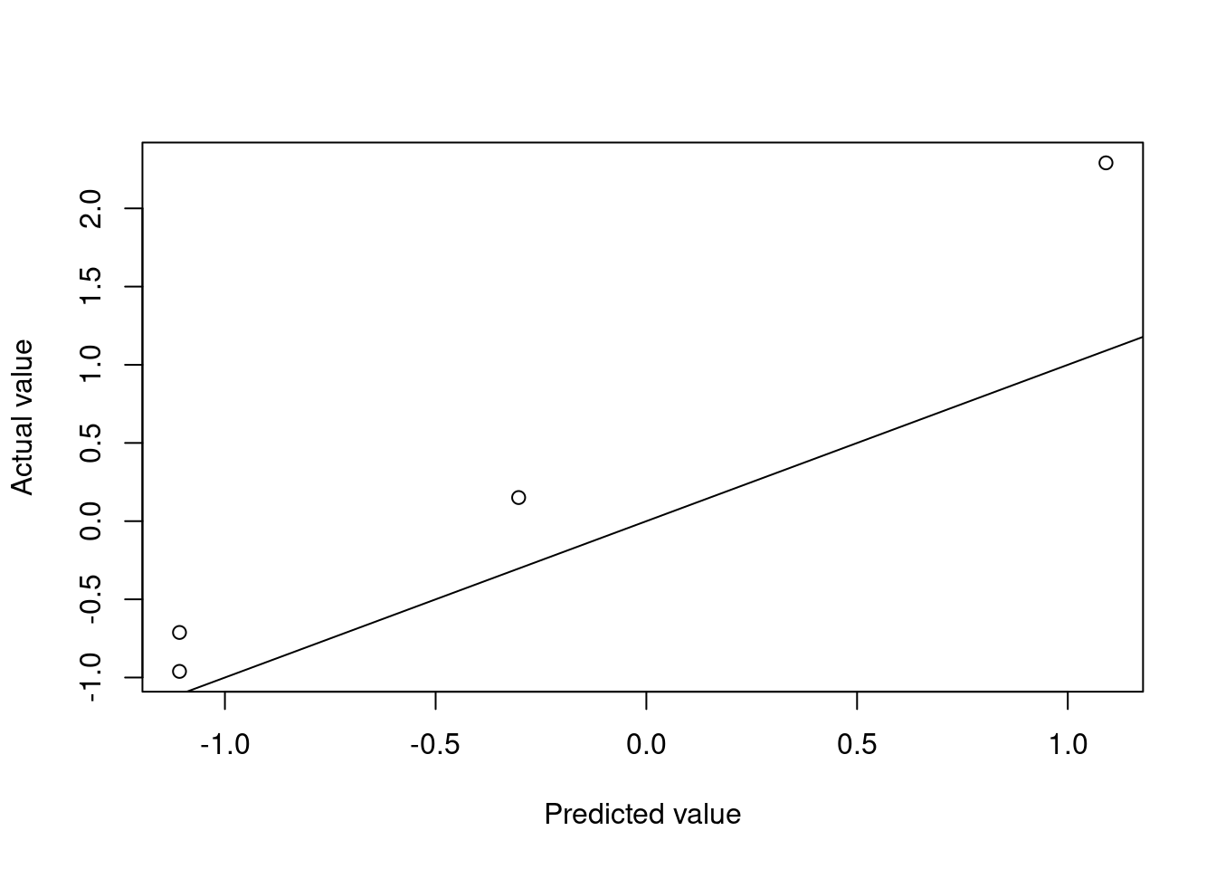
Figure 4.5: Decision tree predictions
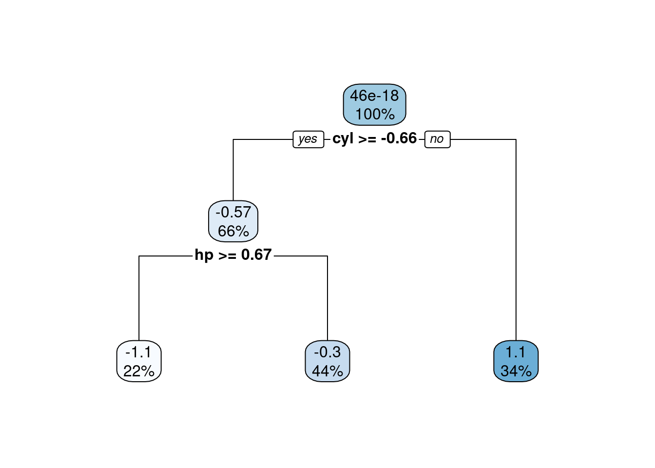
Figure 4.6: Fitted decision tree
4.6 Multivariate Adaptive Regression Splines
The Multivariate Adaptive Regression Spline (MARS) method is a non-parametric regression technique that is based on piecewise linear functions. MARS models are built by recursively partitioning the input space into regions and fitting a linear function to each region. This should sound familiar as it is the same idea as decision trees. The difference is that the MARS model is built from simple linear functions, while the decision tree model is built from constant functions.
We write the MARS model in terms of hinge functions, which are piecewise linear functions that are used to create the piecewise linear functions in the MARS model: \[ f({\mathbf{x}}) = \beta_0 + \sum_{j=1}^{m} \beta_j h_j({\mathbf{x}}), \] where the \(\beta_j\) are the model parameters and the \(h_j({\mathbf{x}})\) are the hinge functions. The hinge functions are defined as \[ h_j({\mathbf{x}}) = \max(0, x_k - c_j) \quad \text{or} \quad \max(0, c_j - x_k), \] where \(x_k\) is one of the input variables and \(c_j\) is the knot point. The “or” here allows us to have functions with negative or positive gradients. The MARS model is built by adding hinge functions to the model and selecting the most important hinge functions. This means that we need to estimate the location of the knot points and the coefficients of the hinge functions. In practice, the knot locations are determined in a manner akin to the decision tree algorithm.
The MARS model is often trained by considering reductions in RMSE. At each stage of the algorithm, the model is trained by adding a hinge function that reduces the RMSE the most. The algorithm is stopped when the RMSE is no longer reduced by adding a hinge function.
The MARS model has the advantage of being interpretable because the model is built from simple linear functions. Figure 4.7 shows an example of the MARS model in one dimension.
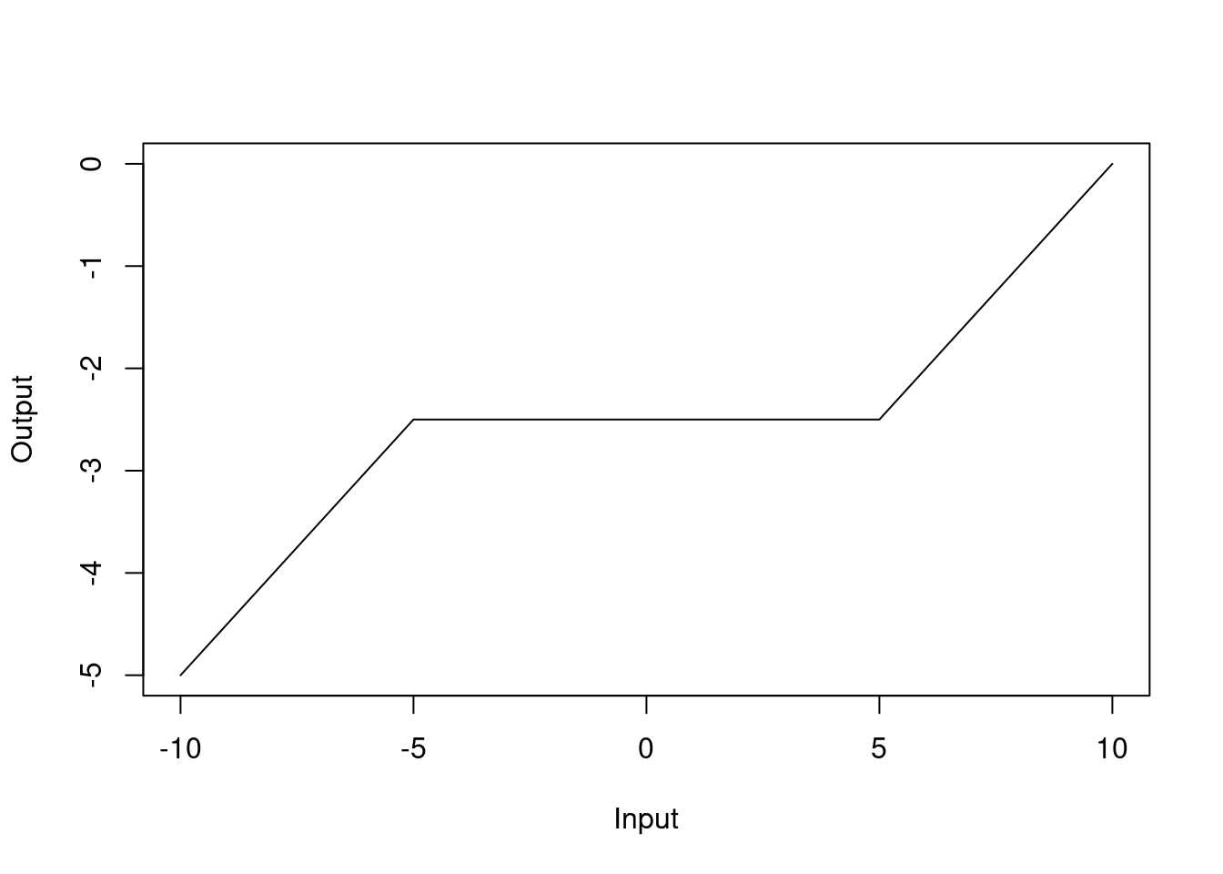
Figure 4.7: MARS model in one dimension
Example
We fit a MARS model to the Boston data set using the earth package within caret.
library(earth)

set.seed(123)
mars.fit.Boston <- train(medv ~ .,
                         data = Boston,
                         method = "earth",
                         trControl = trainControl(method = "cv",
                                                  number = 10),
                         tuneGrid = expand.grid(degree = 1:2,
                                                nprune = 2:10))

summary(mars.fit.Boston)
## Call: earth(x=matrix[506,13], y=c(0.1595,-0.101...), keepxy=TRUE, degree=2,
## nprune=10)
##
## coefficients
## (Intercept) 0.1549343
## h(rm-0.208315) 0.9102939
## h(-1.15797-dis) 15.7464951
## h(lstat- -0.914859) -0.5632729
## h(1.36614-nox) * h(lstat- -0.914859) 0.1849062
## h(0.206892-rm) * h(dis- -1.15797) -0.1600934
## h(rm-0.208315) * h(ptratio-0.0667298) -1.3843533
## h(-0.612548-tax) * h(-0.914859-lstat) 3.8341243
## h(tax- -0.612548) * h(-0.914859-lstat) 2.8353130
##
## Selected 9 of 27 terms, and 6 of 13 predictors (nprune=10)
## Termination condition: Reached nk 27
## Importance: rm, lstat, ptratio, tax, dis, nox, crim-unused, zn-unused, ...
## Number of terms at each degree of interaction: 1 3 5
## GCV 0.137542 RSS 63.93938 GRSq 0.8627298 RSq 0.8733874In the model summary, the h() functions are the hinge functions that are used to create the piecewise linear functions. For instance, h(rm-0.208315) with a coefficient of 0.91 should be interpreted as the hinge function \(\max(0, rm-0.208315)\), which can be visualised as
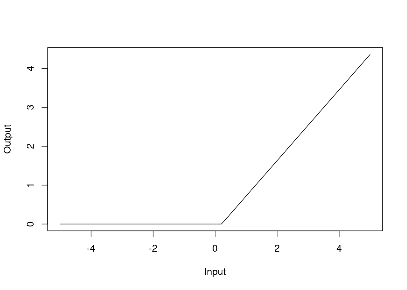
Figure 4.8: Hinge function for rm variable
Similarly, h(-1.15797-dis) with a coefficient of 15.7 should be interpreted as the hinge function \(\max(0, -1.15797-dis)\):
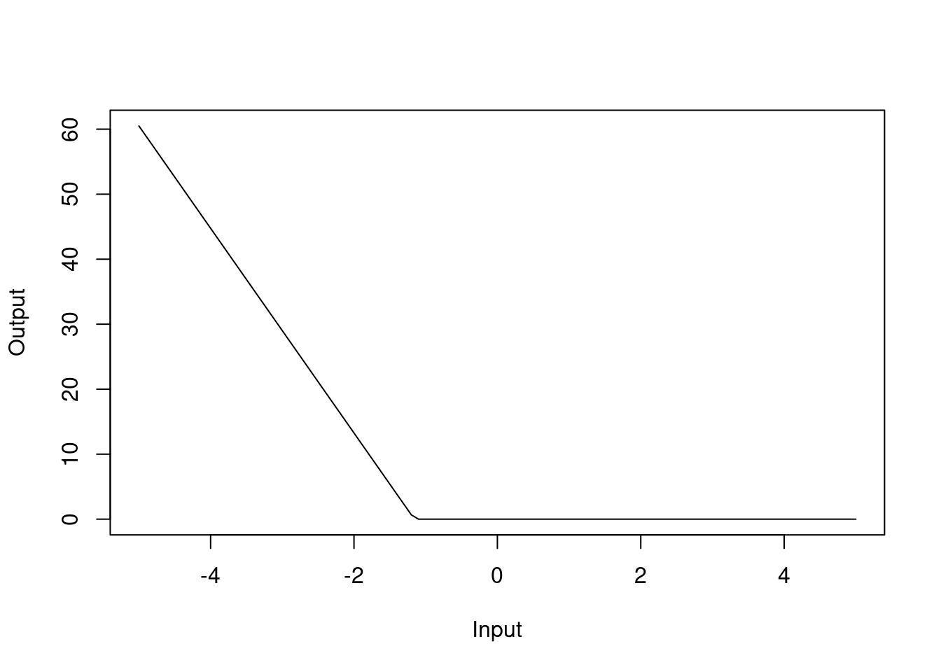
Figure 4.9: Hinge function for dis variable
The MARS model has a RMSE of 0.41. In the model summary, we can see that we have selected 9 of 27 terms and 6 of the 13 predictors have been used. This means that the MARS model has selected 9 hinge functions for the final model that utilise 6 of the 13 explanatory variables. Like in the standard linear regression case, rm, dis and lstat are important predictors in the MARS model.