Chapter 3 Supervised Learning — Classification
3.1 Historical notes
Classification applications have a long history in statistics and machine learning. The first ML classification algorithm was the perceptron, which we will meet later, invented in 1943 by Warren McCulloch and Walter Pitts and developed for practical use by Frank Rosenblatt in 1957. In statistics, classification has a much longer history with examples dating back to the 19th century. The most famous example is Fisher’s iris dataset, which was used to develop the Fisher’s linear discriminant analysis (as we have seen). Fisher’s LDA is still used today in many applications, such as facial recognition and handwriting recognition. Another common technique in statistics is logistic regression, which is a linear classifier that uses a logistic function to classify inputs into two categories. With origins in the 1800s and turned into the statsitical tool it is today in the middle of the 1900s, logistic regression is widely used in many applications, such as credit scoring and medical diagnosis.
The general idea behind classification is to learn a function that maps inputs to categories. The function is learnt from a training dataset, which consists of input-output pairs. The function is then used to classify new inputs into one of the output categories. The training data need to be labelled; that is, the output categories need to be known.
3.2 Running examples
To aid explanations, we will use two well known data sets throughout this chapter.
The first is the aforementioned iris data set. The iris data set consists of 150 observations of iris flowers, with four features (sepal length, sepal width, petal length, petal width) and three classes (setosa, versicolor, virginica). The goal is to classify the flowers into one of the three classes based on the four variables.
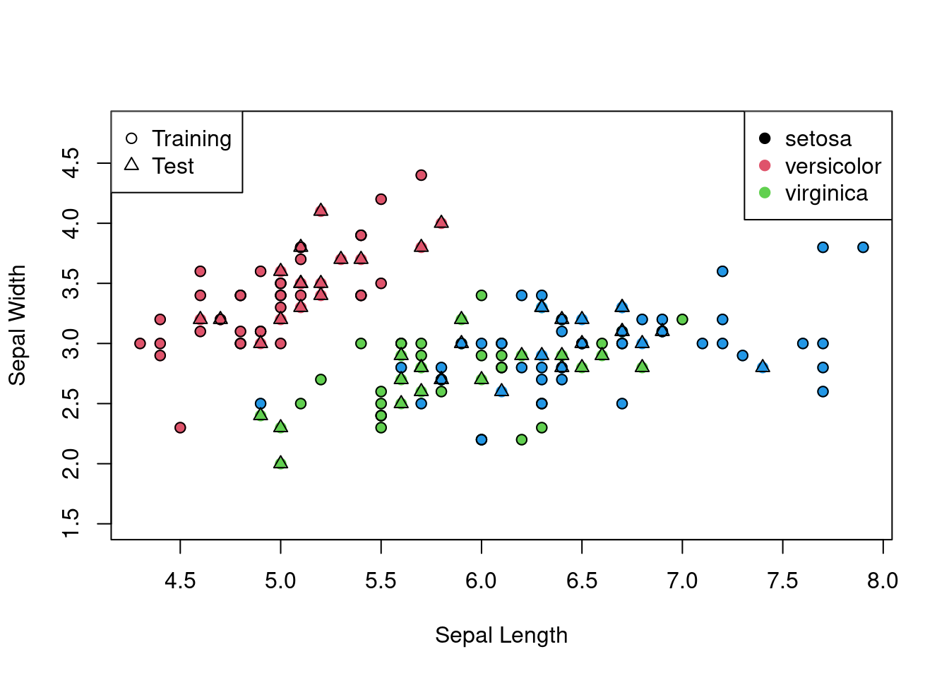
Figure 3.1: The iris data set on the sepal length and width axes with different shapes for test and training and different colours for each class.
Using linear discriminant analysis, we can classify the iris flowers into one of the three classes based on the four variables (as seen in Chapter 1).
The confusion matrix in this example is
| setosa | versicolor | virginica | |
|---|---|---|---|
| setosa | 16 | 0 | 0 |
| versicolor | 0 | 19 | 2 |
| virginica | 0 | 0 | 13 |
For later comparison, we can also calculate the accuracy of the linear discriminant analysis model: 0.96.
Our second running example will be the often cited handwriting recognition data set. Our subset of the handwriting recognition data set consists of thousands observations of handwritten digits, with 784 features (28x28 pixels) and ten classes (0-9). The goal is to classify the digits into one of the ten classes based on the 784 features.
# Load the handwriting datasets
library(readr)
web_url <- "https://www.maths.dur.ac.uk/users/john.p.gosling/MATH3431_practicals/"
MNIST_test <- read_csv(paste0(web_url,
                              "mnist_test_small.csv"))
MNIST_train <- read_csv(paste0(web_url,
                               "mnist_train_small.csv"))

# We don't need all these data for our examples
MNIST_test <- MNIST_test[1:1000, ]
MNIST_train <- MNIST_train[1:2000, ]
The following table shows us the coverage of the digits in the training and test sets.
| Digit | Training | Test |
|---|---|---|
| 0 | 191 | 85 |
| 1 | 220 | 126 |
| 2 | 198 | 116 |
| 3 | 191 | 107 |
| 4 | 214 | 110 |
| 5 | 180 | 87 |
| 6 | 200 | 87 |
| 7 | 224 | 99 |
| 8 | 172 | 89 |
| 9 | 210 | 94 |
Figure 4.2 shows the first digit in the test set.
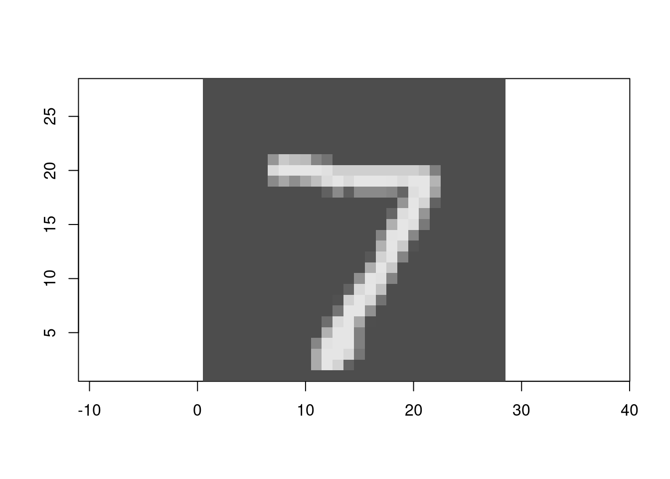
Figure 3.2: The first digit in the test set.
3.3 \(k\)-nearest neighbours
The \(k\)-nearest neighbours algorithm is a simple and intuitive classification algorithm that is widely used in many applications. The algorithm works by finding the nearest neighbours of a new input and classifying the input based on the majority class of the neighbours. The algorithm is non-parametric because it does not make any assumptions about the underlying data distribution. The algorithm is also lazy that means that it does not really learn a function from the training data, but instead stores the training data and uses it to classify new inputs.
3.3.1 Basic algorithm
The \(k\)-nearest neighbours algorithm works as follows:
- Compute the distance between the new input and each training input.
- Sort the distances in ascending order.
- Select the \(k\) nearest neighbours of the new input.
- Classify the new input based on the majority class of the neighbours.
The distance metric used to compute the distances can be any metric, such as Euclidean distance, Manhattan distance, or Minkowski distance. The value of \(k\) can be any positive integer, but is typically chosen to be a number greater than the number of classes to help avoid ties.
The computational cost of this algorithm is in the computing of all the distances and sorting. In practice, implementations of the algorithm use efficient data structures and algorithms to speed up the computation. In particular, the \(k\)-d tree data structure is often used to speed up the computation of the distances.
Example
For this illustration, we will just use two variables from the iris data set: Sepal.Length and Sepal.Width.
# k-nearest neighbours
library(class)

# Compute the distance between the new input
# and each training input
knn_results <- knn(train = train_data[, 1:2],
                   test = test_data[, 1:2],
                   cl = train_data$Species,
                   k = 5)

# Create the confusion matrix
confusion_matrix <- table(knn_results, test_data$Species)
confusion_matrix
##
## knn_results setosa versicolor virginica
## setosa 16 0 0
## versicolor 0 10 4
## virginica 0 11 9The accuracy here is 0.7. The following plot highlights what the algorithm is doing for a couple of the test points.
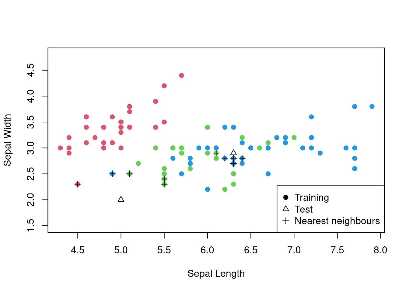
Figure 3.3: The \(k\)-nearest neighbours algorithm in action for the iris data set.
As noted, we are free to utilise any distance metric we wish. Consider the same example as above, but using the Manhattan distance metric.
# k-nearest neighbours with Manhattan distance
knn_results <- NULL

# For each test point
for (i in 1:nrow(test_data)) {
  # Compute the Manhattan distance between the test point
  # and each training point
  distances <- apply(train_data[, 1:2], 1,
                     function(x) sum(abs(x - test_data[i, 1:2])))
  # Find the k nearest neighbours checking for ties
  nearest_neighbours <- train_data[distances <= sort(distances)[5], ]

  # Classify the test point based on the majority
  # class of the neighbours again checking for ties
  candidates <- names(table(nearest_neighbours$Species)[
    table(nearest_neighbours$Species)>=sort(table(nearest_neighbours$Species),
                                            decreasing = TRUE)[1]])
  knn_results[i] <- sample(candidates)[1]
}

# Confusion matrix
confusion_matrix <- table(knn_results, test_data$Species)
confusion_matrix
##
## knn_results setosa versicolor virginica
## setosa 16 0 0
## versicolor 0 8 4
## virginica 0 13 9This is getting worse: the accuracy now is 0.66. Looking back at the plot of the data, we can see that the data is more spread out along the x-axis than the y-axis. This means that the Manhattan distance metric is not a good choice for this data set. The Euclidean distance metric is a better choice because it takes into account the spread of the data along both axes. Also, in this implementation, it is clear that care is needed when deciding how to deal with ties. If there are ties in the distances, then the algorithm will allow all the data points to vote on the classification of the test point. If there are ties in the class vote, then the algorithm will randomly select a class from the tied classes.
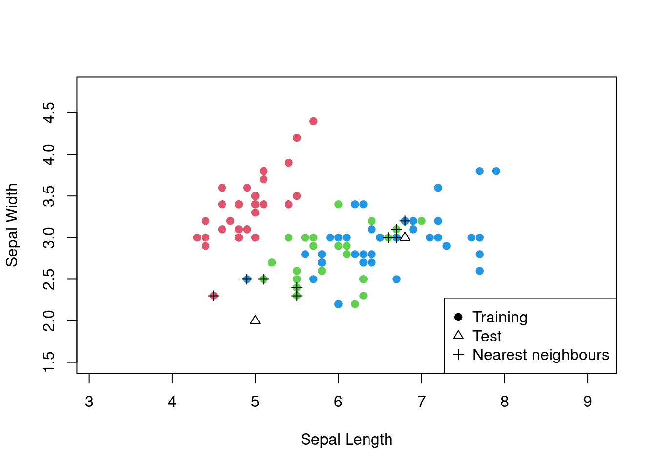
Figure 3.4: The \(k\)-nearest neighbours algorithm in action for the iris data set using the Manhattan distance.
3.4 Naive Bayes classifier
The naive Bayes classifier is another efficient classification algorithm that is widely used in many applications. The algorithm is based on Bayes’s theorem, which is a fundamental theorem in probability theory. The algorithm is called “naive” because it makes the naive assumption that the variables are conditionally independent given the class. This assumption simplifies the computation of the class probabilities and makes the algorithm computationally efficient. The probabilities underpinning the naive Bayes classifier can be written as:
\[ P(y | x_1, x_2, \ldots, x_n) = \frac{P(y) \prod_{i=1}^{n} P(x_i | y)}{P(x_1, x_2, \ldots, x_n)}, \]
where \(y\) is the class label, \(x_1, x_2, \ldots, x_n\) are the features, and \(P(y)\), \(P(x_i | y)\), and \(P(x_1, x_2, \ldots, x_n)\) are the class prior, the feature likelihood, and the evidence, respectively. Now, the non-naive version would look like this:
\[ P(y | x_1, x_2, \ldots, x_n) = \frac{P(y) P(x_1, x_2, \ldots, x_n | y)}{P(x_1, x_2, \ldots, x_n)}. \] The \(P(x_1, x_2, \ldots, x_n | y)\) term is the joint likelihood of the features given the class, which is much more complex to compute than the product of the individual likelihoods.
In practice, the prior \(P(y)\) and the likelihood \(P(x_i | y)\) are estimated from the training data using maximum likelihood estimation. The evidence \(P(x_1, x_2, \ldots, x_n)\) is a constant that does not affect the classification decision and can be ignored. The class label is then assigned to the input with the highest class probability.
More explicitly, the algorithm works as follows:
- Estimate the class prior \(P(y)\) and the feature likelihood \(P(x_i | y)\) from the training data.
- Compute the class probability for each class using Bayes’s theorem for each test set of predictors.
- Assign the class label with the highest probability for each test set of predictors.
The estimate of the class prior is the proportion of the class labels in the training data, while the estimate of the variable likelihood depends on the variable type. For continuous variables, the likelihood is estimated using a normal distribution, and, for categorical variables, the likelihood is estimated using a categorical distribution.
Example
Imagine, we have a data set with two variables and two classes. We can use the naive Bayes classifier to classify the data into one of the two classes.
Here is our rather small data set.
| \(x_1\) | \(x_2\) | \(y\) |
|---|---|---|
| 1.5 | A | Positive |
| 1.7 | B | Positive |
| 1.3 | A | Positive |
| 1.9 | B | Positive |
| 2.1 | A | Positive |
| 2.3 | B | Negative |
| 2.5 | A | Negative |
| 2.7 | B | Negative |
| 1.9 | A | Negative |
We have estimated class prior probabilities of \(P(\text{Positive}) = 5/9\) and \(P(\text{Negative}) = 4/9\).
We have also estimated the likelihoods of the variables as follows:
- \(x_1 | \text{Positive} \sim N(1.7, 0.1)\),
- \(x_1 | \text{Negative} \sim N(2.3, 0.1)\),
- \(x_2 | \text{Positive} \sim \text{Categorical}(P_A = 0.6, P_B = 0.4)\),
- \(x_2 | \text{Negative} \sim \text{Categorical}(P_A = 0.5, P_B = 0.5)\).
Example
Here is the naive Bayes classifier in action for the MNIST data set.
# Naive Bayes
# This library is based on material from a course at TU Wien
library(e1071)

# Convert the digit column to a factor
MNIST_train$label <- as.factor(MNIST_train$label)

# Train the Naive Bayes classifier
naive_bayes_model <- naiveBayes(label ~ .,
                                data = MNIST_train)

# Predict the class labels for the test data
naive_bayes_predictions <- predict(naive_bayes_model,
                                   newdata = MNIST_test)

# Create the confusion matrix
confusion_matrix <- table(naive_bayes_predictions,
                          MNIST_test$label)
confusion_matrix
##
## naive_bayes_predictions 0 1 2 3 4 5 6 7 8 9
## 0 74 0 6 9 5 10 4 2 1 1
## 1 1 125 22 20 10 13 5 24 19 13
## 2 0 0 20 1 0 1 1 0 1 0
## 3 0 0 5 26 0 0 0 1 1 0
## 4 0 0 0 0 18 2 0 2 2 1
## 5 1 0 4 5 0 1 0 1 2 0
## 6 2 1 18 7 12 4 72 1 0 1
## 7 0 0 0 2 1 0 0 29 0 0
## 8 7 0 41 32 26 54 5 13 60 5
## 9 0 0 0 5 38 2 0 26 3 73It can be useful to visualise the confusion matrix as a heat map when there are so many categories.
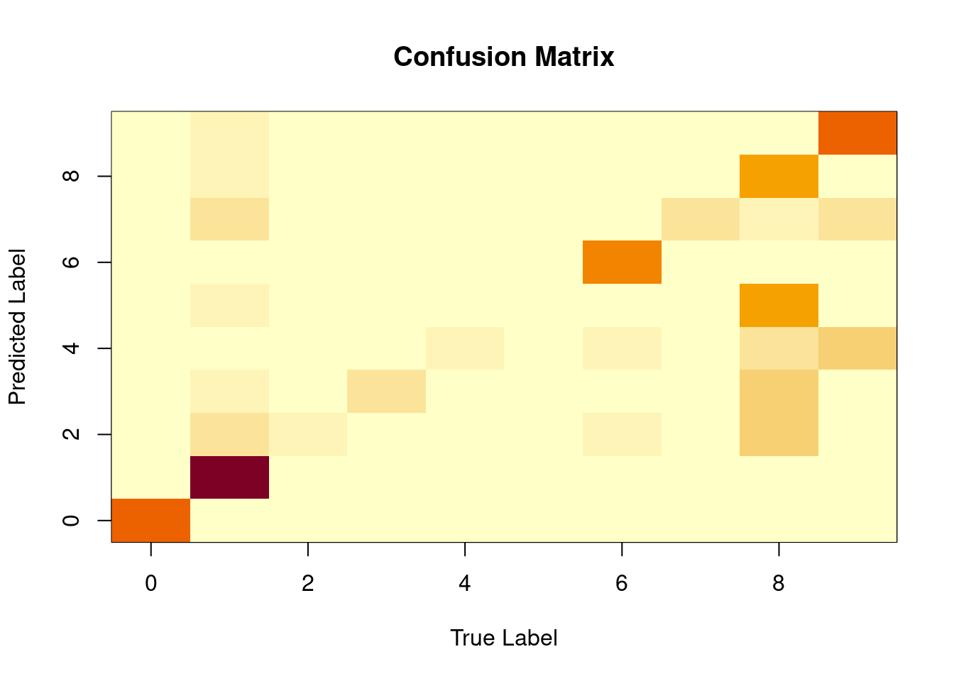
Figure 3.5: The confusion matrix for the MNIST data set from the naive Bayes classifier.
3.5 Decision trees
Decision trees are a popular and powerful classification algorithm that is widely used in many applications. The algorithm works by recursively partitioning the feature space into regions that are homogeneous with respect to the class labels. The algorithm is based on a tree structure, where each node represents a decision based on a feature, and each leaf node represents a class label. The algorithm is simple and intuitive, and it can handle both numerical and categorical features.
The decision tree algorithm works as follows:
Select the best variable to split the data.
Split the data into two subsets based on the variable.
Repeat steps 1 and 2 for each subset until the data is homogeneous with respect to the class labels.
Assign the majority class label to each leaf node.
The algorithm can be used to classify new inputs by traversing the tree from the root node to a leaf node based on the variable values of the input. The class label of the leaf node is then assigned to the input.
What is meant here by the “best variable” or “homogeneous with respect to the class labels”? Essentially, we want the data in each region belongs to a single class so let’s pick the variable where things are most confused in terms of class. This is where the Gini impurity or entropy come in. The Gini impurity is a measure of the impurity of a region, with a value of 0 indicating that the region is pure and a value of 1 indicating that the region is impure. The entropy is a measure of the impurity of a region, with a value of 0 indicating that the region is pure and a value of 1 indicating that the region is impure. The formula for the Gini impurity is:
\[ I_G(t) = 1 - \sum_{i=1}^{c} p(i|t)^2, \]
where \(I_G(t)\) is the Gini impurity of node \(t\), \(c\) is the number of classes, and \(p(i|t)\) is the probability of class \(i\) at node \(t\). The formula for the entropy is:
\[ I_H(t) = - \sum_{i=1}^{c} p(i|t) \log_2 p(i|t), \]
where \(I_H(t)\) is the entropy of node \(t\), \(c\) is the number of classes, and \(p(i|t)\) is the probability of class \(i\) at node \(t\). These probabilities are usually crudely estimated using the class labels of the data points in each region (just like in the naive Bayes classifier).
Example
Let’s consider the digit recognition data set and use the decision tree algorithm to classify the digits into one of the ten classes based on the 784 features.
# Decision tree
library(rpart)

# Train the decision tree
decision_tree_model <- rpart(label ~ ., data = MNIST_train)

# Predict the class labels for the test data
decision_tree_predictions <- predict(decision_tree_model,
                                     newdata = MNIST_test,
                                     type = "class")

# Create the confusion matrix
confusion_matrix <- table(decision_tree_predictions,
                          MNIST_test$label)

# Visualise the confusion matrix
image(0:9,0:9,confusion_matrix,
      xlab="True Label",
      ylab="Predicted Label",
      main="Confusion Matrix")
Figure 3.6: The confusion matrix for the MNIST data set from the decision tree classifier.
We can look at the tree to try to work out how the data are being classified.
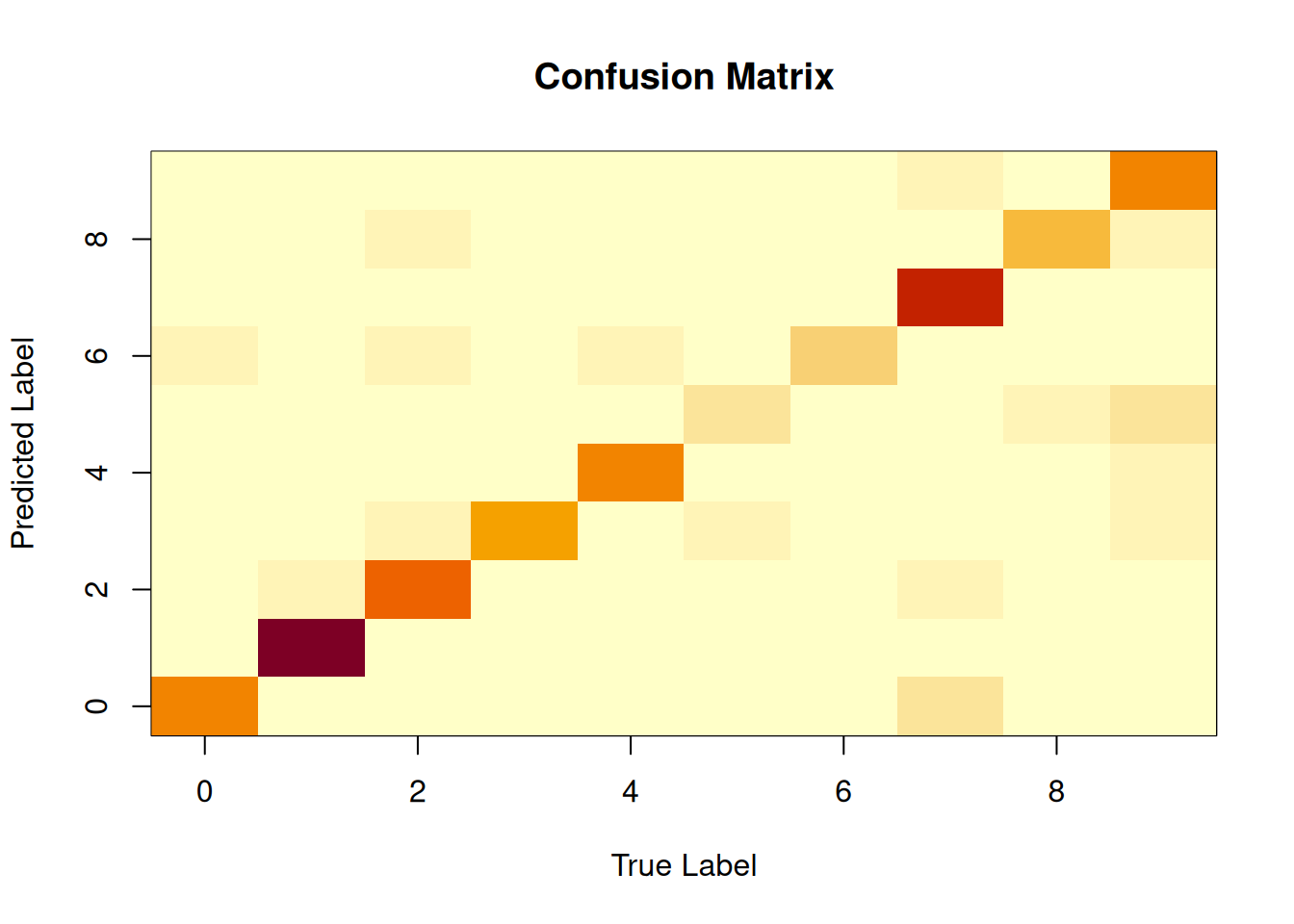
Figure 3.7: The decision tree for the MNIST data set.
If we squint, we can see that the decision tree is essentially asking if a pixel is blank or not. With surprisingly few splits, the tree is able to classify the digits with a high degree of accuracy.
3.6 Perceptron
The perceptron is a linear classifier that uses a threshold function to classify inputs into two categories. The perceptron was the first machine learning algorithm capable of learning from its mistakes, and it was used in early applications of machine learning, such as optical character recognition. The perceptron is a simple and efficient algorithm that is widely used in many applications.
We start with a set of weights assigned to each input variable. The algorithm works by updating the weights of the inputs based on the classification error. The weights are updated using the following update rule: \[ w_{i,t+1} = w_{i,t} + \alpha (y - \widehat{y}_t) x_i, \] where \(w_t\) is the weight vector at iteration \(t\), \(\alpha\) is the learning rate, \(y\) is the true class label, \(\widehat{y}_t\) is the predicted class label, and \(x_i\) is the input variable. The algorithm continues to update the weights until the classification error is minimised. Given the weights, the prediction is made by computing the dot product of the weights and the input variables and applying a threshold function to the result: \[ \widehat{y}_t = \text{sign}\left(\sum_{i=1}^{n} w_t x_i\right), \] where \(\widehat{y}\) is the predicted class label, \(w_i\) is the weight of feature \(i\), \(x_i\) is the input feature, and \(\text{sign}(\cdot)\) is the threshold function that returns 1 if the input is greater than zero and -1 otherwise. We have set the threshold to be zero for ease of computation, but it can be set to any value. Note that, like in linear regression, it is conventional to add a constant term to the input variables.
We can prove that the perceptron algorithm converges to a solution if the data is linearly separable. The proof is based on the fact that the perceptron algorithm updates the weights in the direction of the true class label, which eventually leads to a solution that separates the data into two classes.
Here is the perceptron algorithm in pseudo-code including the update rule and tunable learning rate:
- Initialise the weights to zero.
- Set the learning rate.
- Set the maximum number of iterations.
- Repeat the following steps until the maximum number of iterations is reached:
- For each input in the training data:
- Compute the predicted class label.
- Update the weights based on the classification error.
- Return the weights.
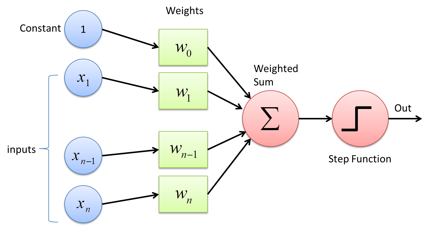
Figure 3.8: The perceptron algorithm
The learning rate comes in to play when we update the weights. The learning rate is a hyperparameter that controls the size of the weight updates. A small learning rate will result in small weight updates, while a large learning rate will result in large weight updates. The learning rate is a critical hyperparameter that can affect the convergence of the algorithm. If the learning rate is too small, the algorithm may take a long time to converge, while if the learning rate is too large, the algorithm may diverge.
The following code shows the perceptron algorithm in action for the iris data set focussing on just two of the species. Here, we use functions in base R to lay bare the algorithm.
# Perceptron
# Use only two species for simplicity
data(iris)
iris <- iris[iris$Species %in% c("setosa", "versicolor"), ]

# Convert the species column to a numeric -1 or 1
iris$Species <- ifelse(iris$Species == "setosa", -1, 1)

# Add in a constant term
iris <- cbind(1, iris)

# Split the iris data set into training and test sets
set.seed(123)
train_index <- sample(1:nrow(iris), 60)
train_data <- iris[train_index, ]
test_data <- iris[-train_index, ]

# Initialise the weights to zero
weights <- rep(0, ncol(iris) - 1)

# Set the learning rate
alpha <- 0.1

# Set the maximum number of iterations
max_iter <- 100

# Repeat the following steps until the maximum number of
# iterations is reached
for (i in 1:max_iter) {
  # For each input in the training data
  for (j in 1:nrow(train_data)) {
    # Compute the predicted class label
    predicted <- ifelse(sum(weights * train_data[j, 1:5]) > 0,
                        1, -1)
    # Update the weights based on the classification error
    weights <- weights + alpha * (train_data[j, 6] - predicted) *
      train_data[j, 1:5]
  }
}

# Display the fitted weights
weights
## 1 Sepal.Length Sepal.Width Petal.Length Petal.Width
## 31 -0.2 -0.16 -0.62 1.36 0.66# Make predictions
predictions <- NULL
for (j in 1:nrow(test_data)) {
predictions[j] <- ifelse(sum(weights[1,] * test_data[j, 1:5]) > 0,
1, -1)
}
# Create the confusion matrix
confusion_matrix <- table(predictions, test_data$Species)
confusion_matrix##
## predictions -1 1
## -1 20 0
## 1 0 20Here, we have the following formula to classify a new input: \[ \begin{aligned} \widehat{y} &= \text{sign}\left(1.36~\mbox{Petal length} + 0.66~\mbox{Petal width}\right.\\&~~~~~~~~~~~~~~~~ \left. - 0.16~\mbox{Sepal length} -0.62~\mbox{Sepal width} - 0.2\right), \end{aligned} \] where \(\widehat{y}\) is the predicted class label, \(w_i\) is the weight of feature \(i\), \(x_i\) is the input feature, and \(\text{sign}(\cdot)\) is the threshold function that returns 1 if the input is greater than zero and -1 otherwise.
The perceptron is a linear classifier, meaning that it can only reliably classify inputs that are linearly separable. In the second half of this module, you will be introduced to the multi-layer perceptron, which is a non-linear classifier that can classify inputs that are not linearly separable and the kernel trick, which is a technique that can be used to transform the input space into a higher-dimensional space where the inputs are linearly separable.
We should also note that we have set up the perceptron with a step activation function. This is a binary classifier, but we can extend this to a probabilistic classifier by choosing a different activation function. The most common choice is the sigmoid function, which maps the output to the range [0, 1]. (This is the basis of logistic regression.)
Another important extension is to consider multiple classes. The perceptron can be extended to handle multiple classes by using a one-vs-all approach, where a separate perceptron is trained for each class and the class with the highest “score” is selected as the predicted class. The score is computed as the dot product of the weights and the input features.
Example
Here is the perceptron in action for the full iris data set. This time, we will need to consider how to handle multiple classes.
# Perceptron
data(iris)

# Convert the species column to a numeric -1 or 1
# over three columns
iris$setosa <- ifelse(iris$Species == "setosa", 1, -1)
iris$versicolor <- ifelse(iris$Species == "versicolor", 1, -1)
iris$virginica <- ifelse(iris$Species == "virginica", 1, -1)

# Add in a constant term
iris <- cbind(1, iris)

# Split the iris data set into training and test sets
set.seed(123)
train_index <- sample(1:nrow(iris), 60)
train_data <- iris[train_index, ]
test_data <- iris[-train_index, ]

# Initialise the weights to zero
weights <- NULL
weights[[1]] <- rep(0, ncol(iris) - 4)
weights[[2]] <- rep(0, ncol(iris) - 4)
weights[[3]] <- rep(0, ncol(iris) - 4)

# Set the learning rate
alpha <- 0.1

# Set the maximum number of iterations
max_iter <- 100

predicted <- NULL
# Repeat the following steps until the maximum number of
# iterations is reached
for (i in 1:max_iter) {
  # For each input in the training data
  for (j in 1:nrow(train_data)) {
    # Compute the predicted class label
    for (k in 1:3) {
      predicted[k] <- ifelse(sum(weights[[k]] * train_data[j, 1:5]) > 0,
                             1, -1)
    }
    # Update the weights based on the classification error
    for (k in 1:3) {
      weights[[k]] <- weights[[k]] + alpha *
        (train_data[j, 6 + k] - predicted[k]) * train_data[j, 1:5]
    }
  }
}

# Calculate the scores from each class
scores <- matrix(0, nrow = nrow(test_data), ncol = 3)
for (j in 1:nrow(test_data)) {
  for (k in 1:3) {
    scores[j, k] <- sum(weights[[k]] * test_data[j, 1:5])
  }
}

# Predict class based on largest score
predictions <- apply(scores, 1, which.max)

# Convert predictions to class labels
class_labels <- c("setosa", "versicolor", "virginica")
predictions <- class_labels[predictions]

# Create the confusion matrix
confusion_matrix <- table(test_data$Species, predictions)
confusion_matrix
## predictions
## setosa versicolor virginica
## setosa 32 0 0
## versicolor 15 3 12
## virginica 0 1 273.7 Balancing classes
In many classification problems, the classes are imbalanced, meaning that one class has more observations than the other classes. This can lead to biased models that favour the majority class and perform poorly on the minority class. To address this issue, we can balance the classes by using techniques such as oversampling, undersampling, and synthetic data generation.
Here, we will only consider oversampling. Oversampling is a technique that involves duplicating the minority class observations to balance the classes. This can be done by randomly sampling the minority class observations with replacement until the classes are balanced. The oversampling technique can help improve the performance of the model on the minority class and reduce the bias towards the majority class.
Example
Let’s consider a synthetic data set with imbalanced classes and use the oversampling technique to balance the classes.
library(rpart)

# Synthetic data set with imbalanced classes
set.seed(123)
n <- 100
data <- data.frame(x = rnorm(n),
                   y = rnorm(n),
                   class = sample(c(0, 1), n,
                                  replace = TRUE,
                                  prob = c(0.9, 0.1)))

# Visualise the data set
plot(data$x, data$y,
     col = data$class + 1, pch = 19)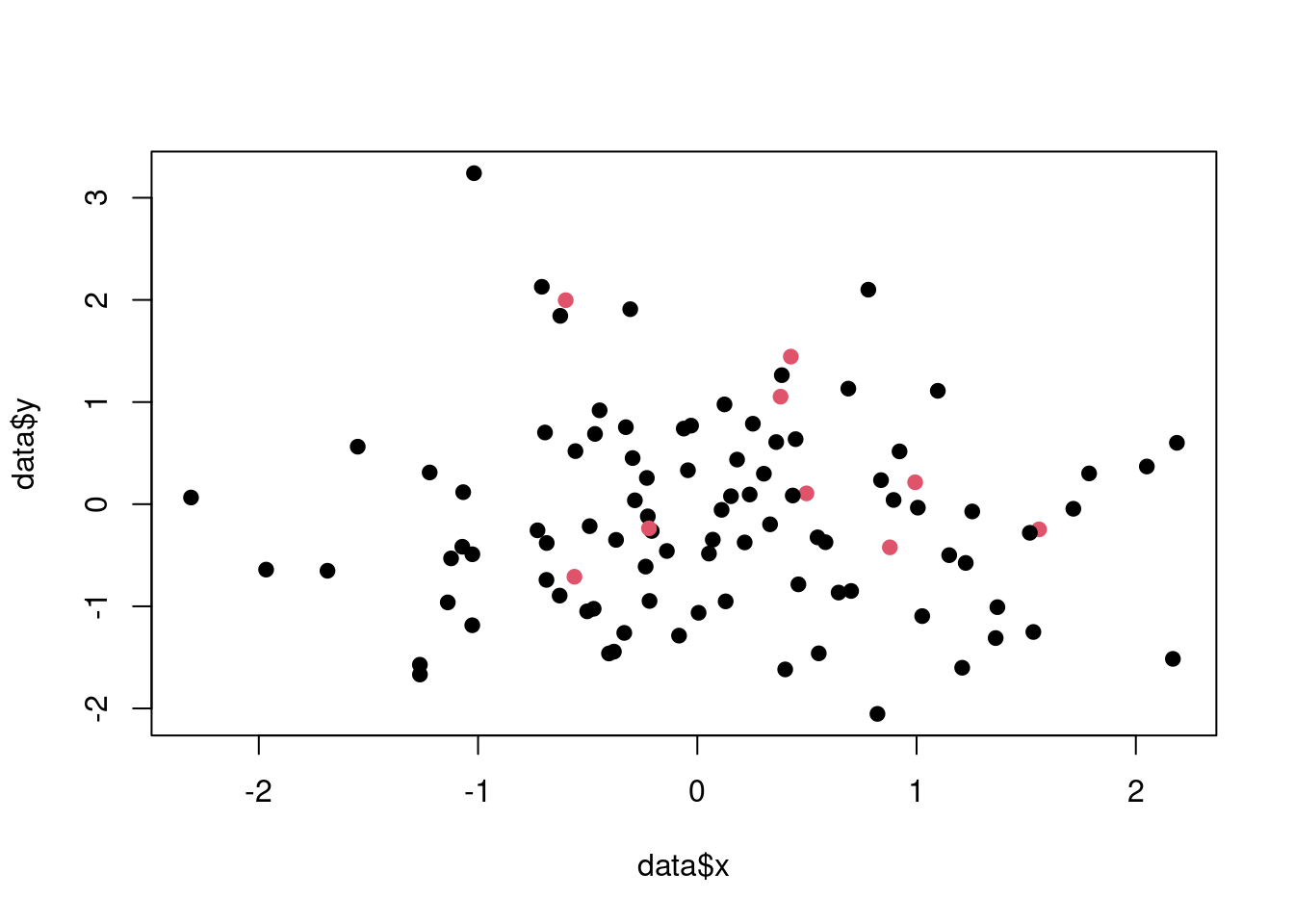
Figure 3.9: The synthetic data set with imbalanced classes.
# Fit a decision tree to the data set
decision_tree_model <- rpart(class ~ .,
                             data = data,
                             method = "class")

# Predict the class labels for the data set
predictions <- predict(decision_tree_model,
                       type = "class")

# Create the confusion matrix
confusion_matrix <- table(predictions, data$class)
confusion_matrix
##
## predictions 0 1
## 0 91 9
## 1 0 0The confusion matrix shows that the model is biased towards the majority class and performs poorly on the minority class. To address this, we can balance the classes using the oversampling technique.
# Oversampling
# Balance the classes using the oversampling technique
n_maj <- sum(data$class == 0)
n_min <- sum(data$class == 1)
data_minority <- data[data$class == 1, ]
data_oversampled <- rbind(data,
                          data_minority[sample(1:n_min,
                                               n_maj - n_min,
                                               replace = TRUE), ])

# Count the number in each class before and after
table(data$class)
##
## 0 1
## 91 9##
## 0 1
## 91 91Now, we can fit a decision tree to the oversampled data set and evaluate the model performance.
# Fit a decision tree to the oversampled data set
decision_tree_model <- rpart(class ~ .,
                             data = data_oversampled,
                             method = "class")

# Predict the class labels for the data set
predictions <- predict(decision_tree_model,
                       newdata = data,
                       type = "class")

# Create the confusion matrix
confusion_matrix <- table(predictions, data$class)
confusion_matrix
##
## predictions 0 1
## 0 74 1
## 1 17 8