Chapter 1 Preliminaries
We will start with some building blocks from statistics so we can start to lay out the notation and ideas that we will use throughout the course.
1.1 Data matrices
We make multiple measurements (\(p\) variables, say) on each of a set of individuals (\(n\), say). Let \(x_{ri}\) by the measurement of the \(i\)th variable on the \(r\)th individual (\(i = 1, \ldots, p, r = 1, \ldots, n\)). In general, \(i, j, k\) will index the variables and \(r, s, t\) will index the individuals.
Arrange the data as an \(n \times p\) matrix \(X = (x_{ri})\) called the data matrix. Each column \(\mathbf{x}_{(i)}\) represents a univariate vector of observations on just one variable: the \(i\)th. Hence, we have that \[ X = \begin{pmatrix} \mathbf{x}_{(1)} \ldots \mathbf{x}_{(p)} \end{pmatrix} \] Each row \(\mathbf{x}_r\) represents the collection of measurements on the \(r\)th individual. \[ X = \begin{pmatrix} \mathbf{x}_1^T \\ \vdots \\ \mathbf{x}_n^T \end{pmatrix}. \]
Note that, we may find that we run into issues of identifiability if \(p > n\). Informally, this means that we have more parameters to find than we have data points, which causes issues if you think back to the idea of solving a set of linear equations. We will discuss this in more detail later.
We will be using the following notation throughout the course to describe the sets of data that we are working with:
\[ \mathcal{Z} = \mathcal{X} \times \mathcal{Y}, \]
where \(\mathcal{Z}\) is the set of all data points, \(\mathcal{X}\) is the set of all input data points (with individual elements usually encoded in a matrix), and \(\mathcal{Y}\) is the set of all output data points (with individual elements encoded in a vector). Like anything in mathematics, there are a number of other conventions for when we refer to elements of \(\mathcal{X}\) and \(\mathcal{Y}\). For instance, we might call them “predictors and responses” or “features and labels” or “independent and dependent variables” instead of “inputs and outputs”.
1.1.1 Sample mean vector
It is useful to have a measure of the central tendency of the data. The sample mean vector is defined as \(\overline{\mathbf{x}}_{p \times 1}\) with \(\overline{x}_i = \frac{1}{n} \sum_{r=1}^n x_{ri}\); that is, the sample mean for variable \(i\).
In matrix terms, \(\overline{\mathbf{x}} = \frac{1}{n} X^T \mathbf{1}_n\) where \(\mathbf{1}_n = \begin{bmatrix} 1, \cdots, 1 \end{bmatrix}^T\).
1.1.2 Sample variance matrix
Similarly, we might want to have a measure of the variability of the data. Unlike the sample mean vector, we need more than just the individual sample variances. We need to know how the variables are related to each other. The sample variance matrix is a \(p \times p\) matrix that contains the sample variances of the variables on the diagonal and the sample covariances between the variables off the diagonal. The sample variance matrix is also known as the sample covariance matrix or the sample var-cov matrix.
Let \(s_{ij}\) be the sample covariance between variables \(i\) and \(j\): \[ s_{ij} = \frac{1}{n-1} \sum_{r = 1}^n \left(x_{ri} - \overline{x}_i\right) (x_{rj} - \overline{x}_j). \] Note that if \(i = j\) this is just the sample variance \(s_{ii}\). Define \(S_{p \times p} = (s_{ij})\) to be the sample variance matrix. If \(S\) is diagonal, all \(p\) variables are uncorrelated.
\(S\) can be defined in matrix form as follows. Let \(H = I - \frac{1}{n} \mathbf{1}_n \mathbf{1}_n^T\) be the centering matrix with \(I\) the \(p\times p\) identity matrix, then \(S = \frac{1}{n-1} X^T H X\).
1.1.3 Correlation matrix
Define the sample correlation matrix \(R\) as \[ R = (r_{ij}) \mbox{ where } r_{ij} = \frac{s_{ij}} {\sqrt{s_{ii} s_{jj}}}, \] that is, the \((i,j)\) element is the sample correlation between variables \(i\) and \(j\). Note that \(r_{ii} = 1\). In matrix form, \(R = D^{-1/2} S D^{-1/2}\) where \(D\) is the diagonal matrix with \(d_{ii} = s_{ii}^{1/2}\).
If \(R = I\), then all \(p\) variables are uncorrelated.
1.1.4 Univariate summaries of variability
Sometimes, it is useful to summarise the variability in a dataset with a single number. When we have multivariate data, we can move from a variance matrix to single number summaries such as the trace of the variance matrix or the determinant of the variance matrix. The trace is a proxy for the total variability in the data (in a additive sense), while the square root of the determinant is a proxy for the volume of the data cloud (the square of this is called the generalised variance).
Here’s a two-dimensional example to illustrate these ideas. We have a random sample drawn from:
\[\begin{align*} X_1&\sim N(0,1),\\ U&\sim N(0,1),\\ X_2&\sim 0.5X_1 + U. \end{align*}\]
We also create a second dataset that is simply both dimensions of the random sample multiplied by 0.5.
The two following plots are scatter plots of the two datasets. The first plot shows the data cloud for the first dataset, while the second plot shows the data cloud for the second dataset. The ellipses are the 90% confidence ellipses for the data clouds.
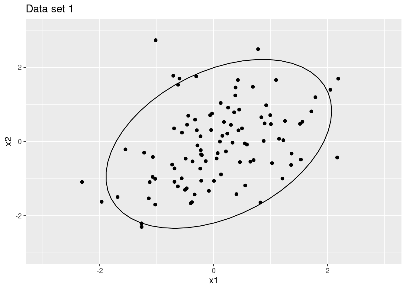
Figure 1.1: Data set 1 with 90% confidence ellipses
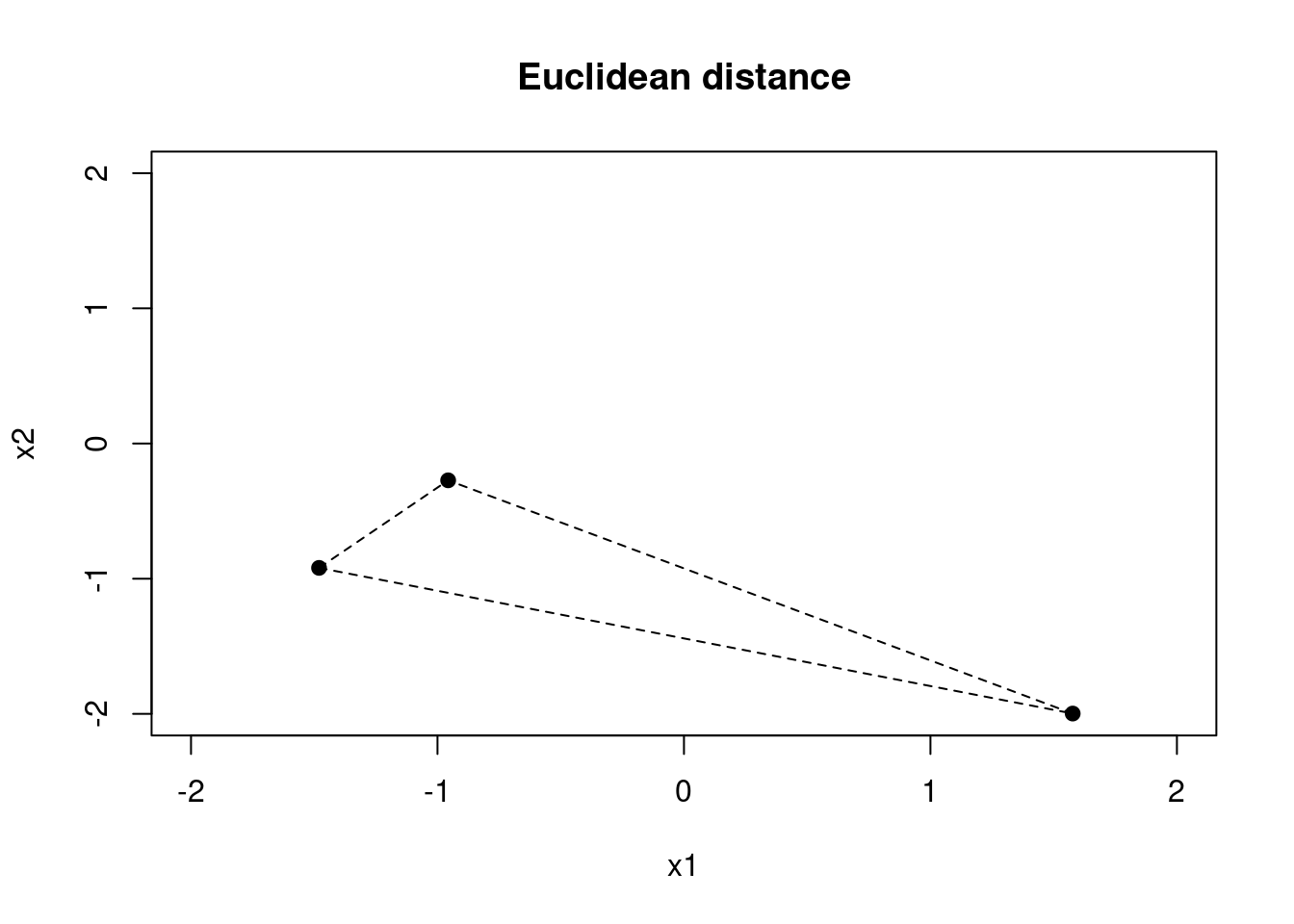
Figure 1.2: Data set 2 with 90% confidence ellipses
For the first dataset, we have a total variance of 1.93 and an approximate volume of 0.88. For the second dataset, we have a total variance of 0.48 and an approximate volume of 0.22, which accords with the transformation used.
1.1.5 Linear combinations
Sometimes it is useful to reduce the dimensionality of a data set by taking linear combinations of the variables. Using matrix notation, we may write \[ Y = X A^T \] where \(X\) is our original data matrix and \(A\) is the transformation matrix. The columns of \(A\) are the linear combinations of the variables.
We can find the sample mean vector of \(Y\) as follows: \[ \overline{\mathbf{y}} = \overline{\mathbf{x}} A^T. \]
Similarly, we can find the sample variance matrix of \(Y\) as follows: \[ S_Y = A S_X A^T. \]
1.1.6 Eigen decomposition
The eigenvectors and eigenvalues of a matrix are important because they can be used to decompose the matrix into simpler components. Recall from linear algebra that the eigenvalues and eigenvectors of a matrix \(S\) are defined by the equation \[ S \mathbf{v} = \lambda \mathbf{v}, \] where \(\mathbf{v}\) is an eigenvector and \(\lambda\) is the corresponding eigenvalue. The eigenvectors of a matrix are orthogonal to each other, and the eigenvalues are real numbers.
Using the definition, we say that the eigen decomposition of a matrix \(S\) is given by \[ S = V \Lambda V^{T}, \] where \(V\) is the matrix of eigenvectors and \(\Lambda\) is the diagonal matrix of corresponding eigenvalues. Loosely speaking, the eigenvectors are the directions in which the data varies the most, while the eigenvalues are the amount of variance in each of these directions.
We then use a linear transformation to rotate the data so that the new variables are uncorrelated. This is useful because it allows us to reduce the dimensionality of the data and to identify the most important variables. We have the following transformation
\[ Y = \left(X - \mathbf{1}_n \overline{\mathbf{x}}^T\right)V^{T}. \]
1.2 Distances between individuals
Let \(\mathbf{x}_r\) and \(\mathbf{x}_s\) be the rows of the data matrix \(X\) for individuals \(r\) and \(s\). We might want a measure of the “distance” between these individuals. Some possibilities that you might have come across are:
- Euclidean distance,
- Pearson distance,
- Mahalanobis distance,
- Manhattan distance.
A distance measure is a type of dissimilarity measure that satisfies the following properties:
- Non-negativity: \(d(\mathbf{x}_r, \mathbf{x}_s) \geqslant 0\) for all \(r\) and \(s\).
- Identity: \(d(\mathbf{x}_r, \mathbf{x}_s) = 0\) if and only if \(\mathbf{x}_r = \mathbf{x}_s\).
- Symmetry: \(d(\mathbf{x}_r, \mathbf{x}_s) = d(\mathbf{x}_s, \mathbf{x}_r)\).
- Triangle inequality: \(d(\mathbf{x}_r, \mathbf{x}_s) + d(\mathbf{x}_s, \mathbf{x}_t) \geqslant d(\mathbf{x}_r, \mathbf{x}_t)\).
Using these properties, we can broaden the sets of objects that we can define distances between. For example, we can define distances between sets, between distributions and between functions.
Distances are important in machine learning because they are used in many algorithms and in the evaluation of models. The flexibility for us to choose which distance metric to use is important because it allows us to tailor the distance metric to the problem at hand and create richer sets of models.
1.2.1 Euclidean distance
The Euclidean distance between individuals \(r\) and \(s\) is given by \[ d(\mathbf{x}_r, \mathbf{x}_s) = \sqrt{\sum_{i=1}^p (x_{ri} - x_{si})^2}. \]
1.2.2 Pearson distance
The Pearson distance between individuals \(r\) and \(s\) is given by \[ d(\mathbf{x}_r, \mathbf{x}_s) = \sqrt{\sum_{i=1}^p \left( \frac{x_{ri} - \overline{x}_i}{s_{ii}} - \frac{x_{si} - \overline{x}_i}{s_{ii}} \right)^2}. \]
Therefore, the Pearson distance is the Euclidean distance between the centred and scaled data.
1.2.3 Mahalanobis distance
The Mahalanobis distance between individuals \(r\) and \(s\) is given by \[ d(\mathbf{x}_r, \mathbf{x}_s) = \sqrt{(\mathbf{x}_r - \mathbf{x}_s)^T S^{-1} (\mathbf{x}_r - \mathbf{x}_s)}. \]
The Malhalanobis distance goes one step further than the Pearson distance by taking into account the correlation between the variables. You can imagine the multiplication by \(S^{-1}\) as a rotation of the data so that we have a new set of variables that are uncorrelated.
1.2.4 Manhattan distance
The Manhattan distance between individuals \(r\) and \(s\) is given by \[ d(\mathbf{x}_r, \mathbf{x}_s) = \sum_{i=1}^p |x_{ri} - x_{si}|. \]
The Manhattan distance is the sum of the absolute differences between the variables.
The Euclidean distance is clearly related to the Manhattan distance. Consider the case where we raise the Manhattan distance to the power of 2. This is equivalent to the Euclidean distance. Hence, we have infinitely many distance metrics that we can use just by choosing different powers.
Example
We can visualise the different distance metrics using a simple example. Let’s consider a two-dimensional example with three individuals.
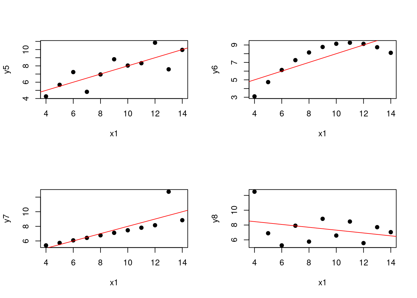
Figure 1.3: Euclidean distance metric for a two-dimensional example
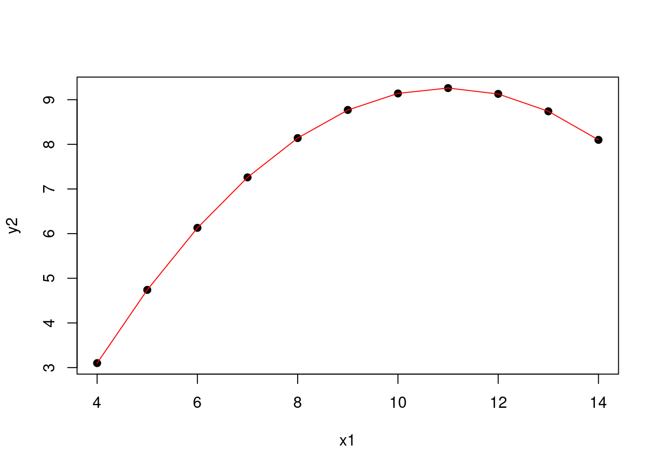
Figure 1.4: Pearson distance metric for a two-dimensional example
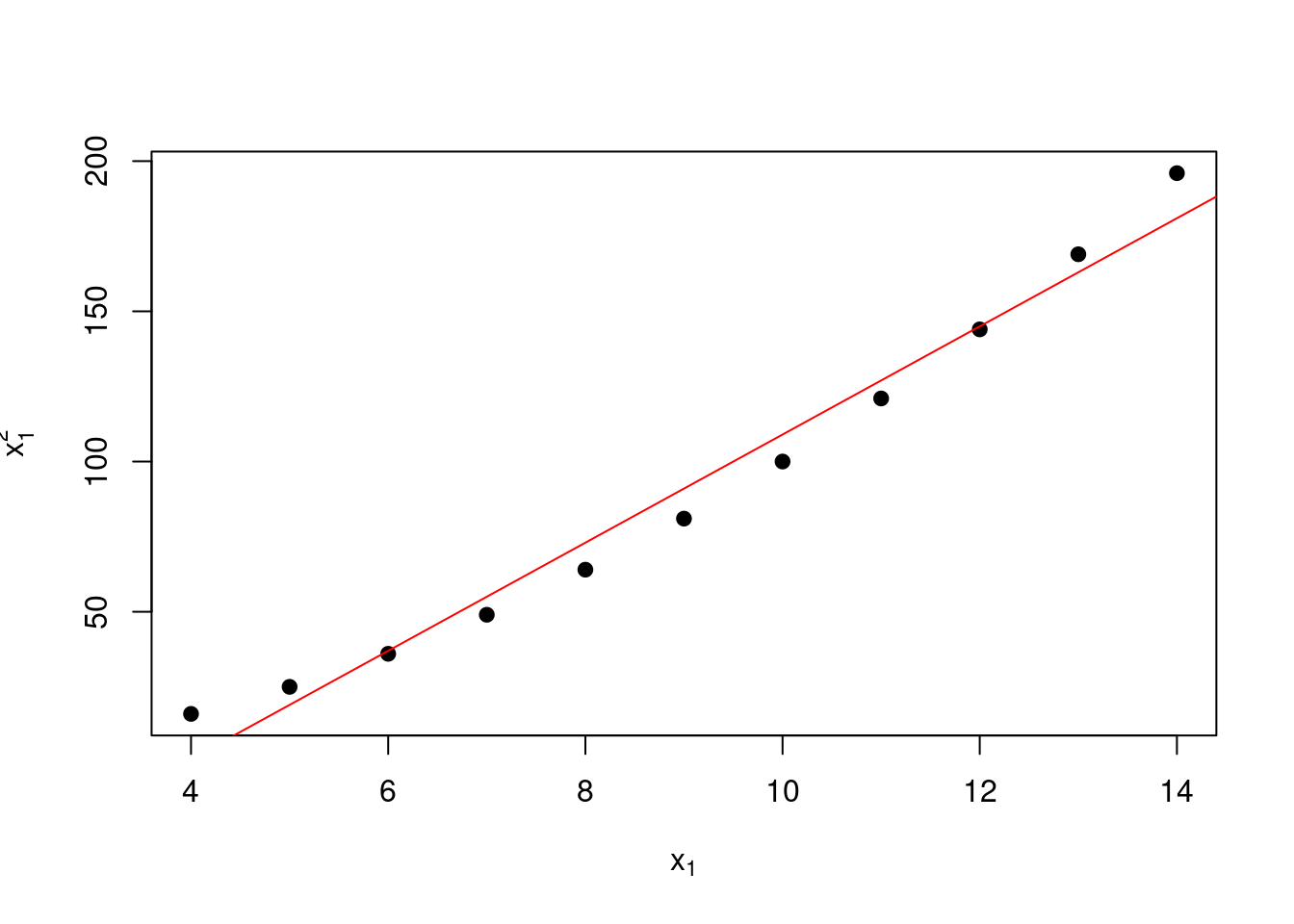
Figure 1.5: Mahalanobis distance metric for a two-dimensional example
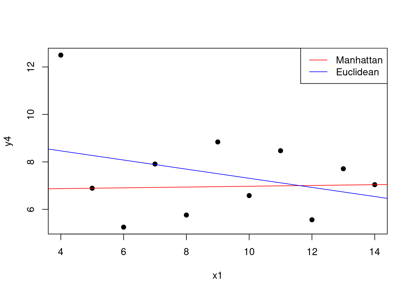
Figure 1.6: Manhattan distance metric for a two-dimensional example
1.2.5 Distances for categorical data
The distance metrics that we have discussed so far are for continuous data. However, we can also define distance metrics for categorical data. The most common distance metric for categorical data is the Hamming distance. In its original from, the Hamming distance is the number of positions at which the corresponding elements are different. For example, the Hamming distance between “2011” and “2001” is 1. For us, it is the number of categorical variables that are different between two individuals. The challenge with this distance metric is that each variable is treated as equally important and there is no notion of relative similarity for each variable. Also, if we have many categorical variables, the Hamming distance can become very large.
We can solve this latter problem by effectively normalising the Hamming distance. We can do this by dividing the Hamming distance by the number of categorical variables. This gives us a distance metric that ranges from 0 to 1. This is related to the idea of the matching coefficient, which is the proportion of variables that are the same between two individuals: our distance is therefore \(1 - \text{matching coefficient}\).
A very popular method for handling the distance between categorical variables involves one hot encoding. This is where we convert the categorical variables into a set of binary variables. For example, if we have a categorical variable with three levels, we can convert this into three binary variables. This allows us to use the Euclidean distance (or whatever distance metric for numerical data we like) between the binary variables. This is a very useful technique because it allows us to use the same distance metric for both numerical and categorical data.
A final metric to consider is the Gower distance, which allows us to weight the variables differently. This is useful because it allows us to account for the fact that some variables are more important than others. The Gower distance is a generalisation of the Hamming distance and the Euclidean distance in that
\[ d(\mathbf{x}_r, \mathbf{x}_s) = \frac{\sum_{i=1}^p w_i d_i(\mathbf{x}_{ri}, \mathbf{x}_{si})}{\sum_{i=1}^p w_i}, \]
where \(w_i\) is the weight for variable \(i\) and \(d_i\) is the distance metric for variable \(i\). In the case where we have all categorical variables, it is usual to use the Hamming distance for \(d_i\). The general form here allows us to use any distance metric for the variables, and opens up possibilities for defining distances between observations that mix numerical and categorical variables.
Example
Let’s consider a simple example with two individuals and two categorical variables. The first individual has the values “A” and “B” for the two variables, while the second individual has the values “A” and “A”. The Hamming distance between the two individuals is 1, while the normalised Hamming distance is 0.5.
If we have a third individual with the values “C” and “C” for the two variables, the Hamming distance between the first and third individuals is 2, while the normalised Hamming distance is 1.
Alternatively, we can consider one hot encoding the variables. The first individual is encoded as (1, 0, 0, 0, 1, 0), while the second individual is encoded as (1, 0, 0, 1, 0, 0). The Euclidean distance between the two individuals is \(\sqrt{2}\). Similarly, the Euclidean distance between the first and third individuals is \(2\).
1.3 Linear regression
The multiple linear regression model with \(p\) predictor variables can be expressed in matrix form as:
\[ \mathbf{y} = \mathbf{X}\beta + \epsilon \]
where:
- \(\mathbf{y}\) is an \(n \times 1\) vector of the response variable
- \(\mathbf{X}\) is an \(n \times (p+1)\) design matrix with a column of ones for the intercept term
- \(\beta\) is a \((p+1) \times 1\) vector of coefficients including the intercept
- \(\epsilon\) is an \(n \times 1\) vector of error terms
More explicitly, the model can be written as:
\[ \begin{pmatrix} y_1 \\ y_2 \\ \vdots \\ y_n \end{pmatrix} = \begin{pmatrix} 1 & x_{11} & x_{12} & \cdots & x_{1p} \\ 1 & x_{21} & x_{22} & \cdots & x_{2p} \\ \vdots & \vdots & \vdots & \ddots & \vdots \\ 1 & x_{n1} & x_{n2} & \cdots & x_{np} \end{pmatrix} \begin{pmatrix} \beta_0 \\ \beta_1 \\ \vdots \\ \beta_p \end{pmatrix} + \begin{pmatrix} \epsilon_1 \\ \epsilon_2 \\ \vdots \\ \epsilon_n \end{pmatrix} \]
The least-squares estimator of \(\beta\) is given by:
\[ \widehat{\beta} = (\mathbf{X}^T\mathbf{X})^{-1}\mathbf{X}^T\mathbf{y} \]
This estimator is obtained by minimising the sum of squared residuals with respect to \(\beta\).
Aside: deriving the least squares estimator
The least squares estimator is derived by minimising the sum of squared residuals. The sum of squared residuals is given by \[ \sum_{i=1}^n (y_i - \widehat{y}_i)^2 = \sum_{i=1}^n (y_i - \mathbf{x}_i^T \beta)^2 = (\mathbf{y} - \mathbf{X}\beta)^T(\mathbf{y} - \mathbf{X}\beta). \] To find the \(\beta\) vector that minimises this expression, we differentiate with respect to \(\beta\) and set the result to zero. The derivative is \[ \nabla_\beta(\mathbf{y} - \mathbf{X}\beta)^T(\mathbf{y} - \mathbf{X}\beta) = -2\mathbf{X}^T(\mathbf{y} - \mathbf{X}\beta). \] Setting this to zero gives \[ \begin{aligned} -2\mathbf{X}^T(\mathbf{y} - \mathbf{X}\widehat{\beta}) &= 0, \\ \mathbf{X}^T\mathbf{y} &= \mathbf{X}^T\mathbf{X}\widehat{\beta}, \\ \widehat{\beta }&= (\mathbf{X}^T\mathbf{X})^{-1}\mathbf{X}^T\mathbf{y}. \end{aligned} \]
This is subject to the technical condition that \(\mathbf{X}^T\mathbf{X}\) is invertible. If we have colinearity in the explanatory variables, this matrix will not be invertible.
We might notice that this estimator is related to the covariance matrix of the centred data: recall that \((n-1) S = X^T H X\). This estimator gives rise to residuals that have some important properties (as we will see later): first, we have \[ \epsilon^T \mathbf{1}_n = 0, \] and, secondly, we have \[ X \epsilon = 0. \] The first property speaks to a balance in the residuals, while the second property speaks to the residuals being orthogonal to the columns of \(X\). This is important because it means that the residuals are uncorrelated with the predictors.
Example
Let’s consider the Anscombe dataset. The Anscombe dataset consists of four sets of data points, each with two variables. The goal is to fit a linear regression model to each set of data points and compare the results.
# Load the Anscombe dataset
data(anscombe)

# Plot the Anscombe dataset
par(mfrow = c(2, 2))
for (i in 5:8) {
  plot(anscombe$`x1`, anscombe[[i]],
       xlab = "x1", ylab = paste0("y", i), pch = 19)
  abline(lm(anscombe[[i]] ~ anscombe$`x1`),
         col = "red")
}
(#fig:1.anscombe.plot)Linear fits for the Anscombe dataset
We can see that the linear regression model fits the data well for the first set of data points in that their is an upward trend plus some noise. However, the linear regression model does not fit the data well for the other sets of data points. For the third and fourth data sets, there is a problem with a single outlier. For the second data set, the relationship between the variables is non-linear that is much more problematic.
However, linear regression does not just mean fitting a straight line to the data. We can also fit a polynomial to the data. For example, we can fit a quadratic model to the second set of data points.
# Fit a quadratic model to the second set of data points
quadratic_model <- lm(y2 ~ poly(x1, 2), data = anscombe)
# summary(quadratic_model)

# Plot the quadratic model
plot(anscombe$`x1`, anscombe$y2,
     xlab = "x1", ylab = "y2", pch = 19)
lines(sort(anscombe$`x1`),
      predict(quadratic_model, data.frame(x1 = sort(anscombe$`x1`)),
              type = "response"),
      col = "red")
Figure 1.7: Quadratic model for the second set of data points
This model is still linear in the sense that we have a linear combination of the various explanatory variables. Here, the expanded form of the model is
\[ y_2 = \beta_0 + \beta_1 x_1 + \beta_2 x_1^2 + \epsilon, \]
and \(x_1^2\) is just another variable that we have created. (This is a general idea in statistics and machine learning: we can create new variables from the existing variables to capture more complex relationships.) We should worry a little about colinearity between the variables: essentially, when we have two variables that are highly correlated, we can have issues with the estimation of the coefficients because we do not know which variable deserves the credit for the prediction.
In this case, we calculate the correlation between \(x_1\) and \(x_1^2\) to be 0.99. This is a high correlation, which is not surprising because we have created \(x_1^2\) from \(x_1\) and the near-straight line relationship between \(x_1\) and \(x_1^2\) over the range of interest that can be seen in the following plot.
# Plot the relationship between x1 and x1^2
plot(anscombe$x1, anscombe$x1^2,
     xlab = expression(x[1]), ylab = expression(x[1]^2),
     pch = 19)

# Add a straightline fit
abline(lm(x1^2 ~ x1,
          data = anscombe),
       col = "red")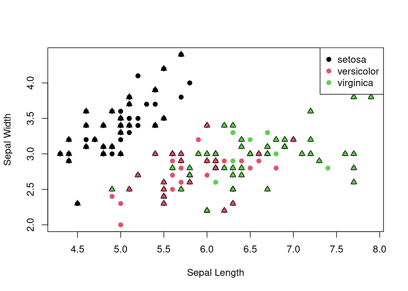
Figure 1.8: Correlation between \(x_1\) and \(x_1^2\)
1.3.1 Using different distance metrics
The fitting of the linear model is usually based on the least squares criterion. This criterion is equivalent to minimising the Euclidean distance between the observed and predicted values. However, we can use different distance metrics to fit the model. For example, we can use the Manhattan distance to fit the model.
# Fit the linear model using the Manhattan distance

# Define a function that calculates the MAE
# between the observed and predicted values
mae <- function(y, y_hat) {
  return(sum(abs(y - y_hat)))
}

# Define a function that returns MAE for
# a vector of coefficients
mae_coefficients <- function(beta) {
  y_hat <- anscombe$`x1` * beta[2] + beta[1]
  return(mae(anscombe$y4, y_hat))
}

# Minimise the MAE
mae_model <- optim(c(0, 0), mae_coefficients)
mae_model$par
## [1] 6.80666450 0.01666688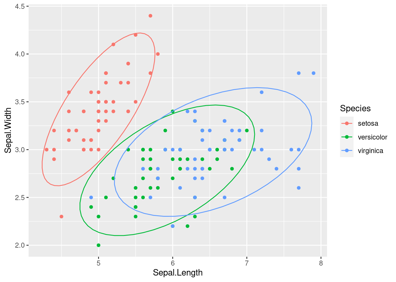
Figure 1.9: Manhattan vs Euclidean distance for the linear model
1.3.2 Partitioning of variance
In linear regression with multiple variables, the total variance in the response variable \(y\) can be partitioned into components associated with the predictor variables and the residual variance. This partitioning is known as the analysis of variance (ANOVA) for the regression model.
Let \(\mathrm{SSR}\) denote the sum of squared residuals:
\[ \mathrm{SSR} = \sum_{i=1}^{n} (y_i - \widehat{y}_i)^2 = \left|\left| \mathbf{y} - \widehat{\mathbf{y}} \right|\right|_2^2 \]
where \(\widehat{y}_i\) is the fitted value of the response variable for observation \(i\).
Furthermore, let \(\mathrm{SST}\) denote the total sum of squares:
\[ \mathrm{SST} = \sum_{i=1}^{n} (y_i - \overline{y})^2 = \left|\left| \mathbf{y} - \overline{\mathbf{y}} \right|\right|_2^2 \]
where \(\overline{y}\) is the mean of the response variable.
The total sum of squares \(\mathrm{SST}\) can be partitioned into two components:
\[ \mathrm{SST} = \mathrm{SSR} + \mathrm{SSM} \]
where \(\mathrm{SSM}\) is the sum of squares due to the regression model (or the explained sum of squares):
\[ \mathrm{SSM} = \sum_{i=1}^{n} (\widehat{y}_i - \overline{y})^2 = \left|\left| \widehat{\mathbf{y}} - \overline{\mathbf{y}} \right|\right|_2^2. \]
This partitioning allows us to quantify the proportion of variance in the response variable that is explained by the predictor variables in the regression model.
The coefficient of determination, \(R^2\), is defined as:
\[ R^2 = \frac{\mathrm{SSM}}{\mathrm{SST}} = 1 - \frac{\mathrm{SSR}}{\mathrm{SST}} \]
\(R^2\) represents the proportion of the total variance in the response variable that is explained by the regression model. It ranges from 0 to 1, with higher values indicating a better fit of the model to the data.
These ideas are closely linked to the bias-variance trade-off. Often we use the difference between the actual values and predicted values to evaluate the model, such prediction error can in fact be decomposed into three parts:
- Bias: The difference between the average prediction of our model and the correct value which we are trying to predict. Model with high bias pays very little attention to the training data and oversimplifies the model. It always leads to high error on training and test data.
- Variance: Variance is the variability of model prediction for a given data point or a value which tells us how uncertainty our model is. Model with high variance pays a lot of attention to training data and does not generalize on the data which it hasn’t seen before. As a result, such models perform very well on training data but has high error rates on test data.
- Noise: Irreducible error that we cannot eliminate.
The bias-variance trade-off explains the situation where we are adding just noise by adding complexity to the model. The training error goes down as the model complexity increases, but the test error is at its minimum when the model complexity is at the right level. We can create a graphical visualisation of bias and variance using a bulls-eye diagram. Imagine that the center of the target is a model that perfectly predicts the correct values. As we move away from the bulls-eye, our predictions get poorer.
We can plot four different cases representing combinations of both high and low bias and variance.
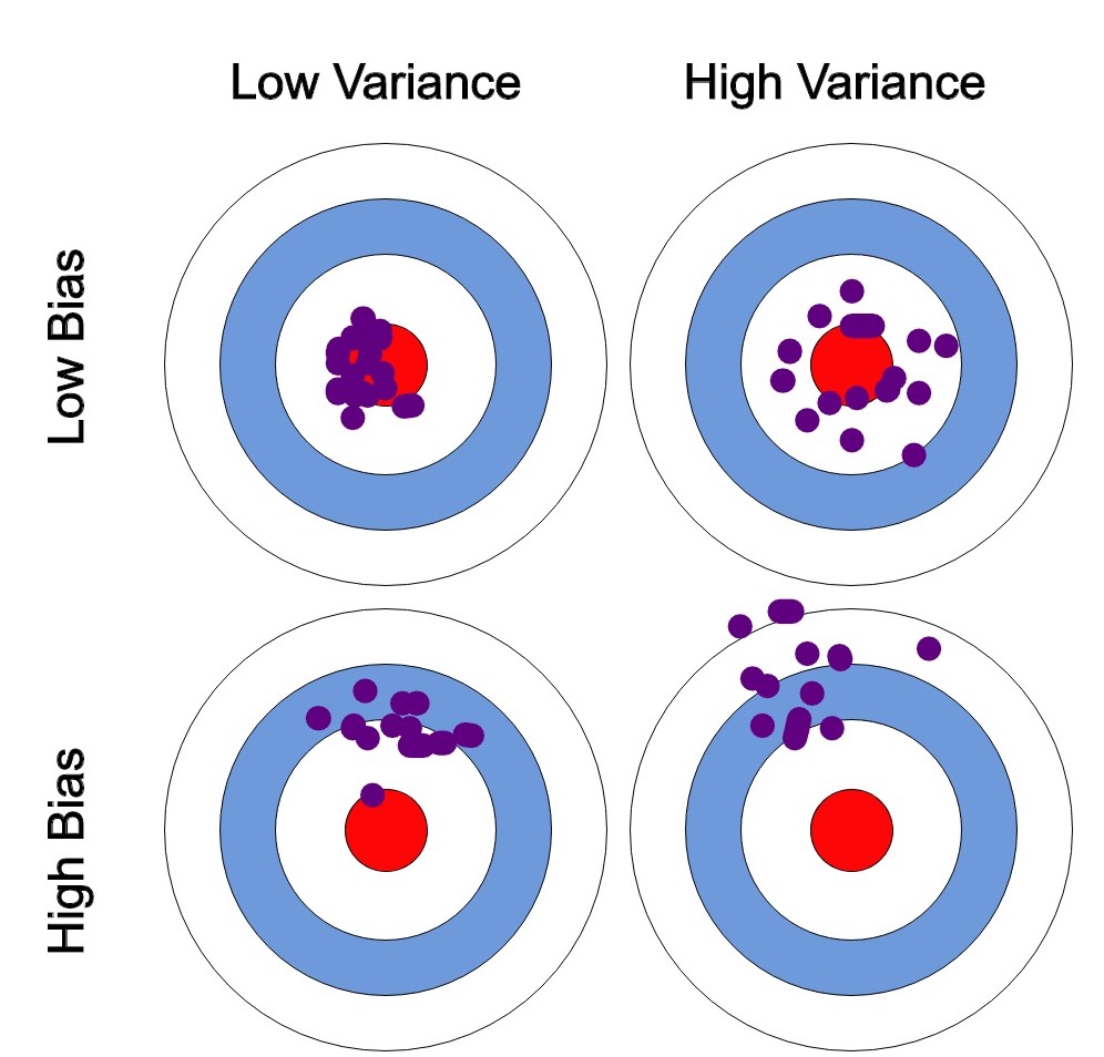
Figure 1.10: Bias-variance trade-off
1.4 Linear discriminant analysis
Linear discriminant analysis (LDA) is a method used in statistics, pattern recognition and machine learning to find a linear combination of features that characterises or separates two or more classes of objects or events. The resulting combination may be used as a linear classifier, or, more commonly, for dimensionality reduction before later classification. LDA was originally proposed by R.A. Fisher in 1936, but the generalisation to more than two classes was not published until 1948 and is attributed to C.R. Rao.
In LDA, we want to find the linear combination of the variables that maximises the ratio of the between-class variance to the within-class variance. The between-class variance is the variance between the classes, while the within-class variance is the variance within each class. The ratio of these two variances is maximised when the classes are well separated.
The LDA method can be broken down into the following steps:
Compute the \(p\)-dimensional mean vector for each of the classes from the dataset.
Compute the variance matrices (within-class and between-class matrices).
Compute the eigenvectors and corresponding eigenvalues for the matrices.
Sort the eigenvectors by decreasing eigenvalues and choose \(k\) eigenvectors with the largest eigenvalues to form a \(p \times k\) dimensional matrix \(W\) (where every column represents an eigenvector).
Use this \(p \times k\) eigenvector matrix to transform the samples onto the new subspace. This can be summarised by the matrix multiplication: \(U = X \times W\) (where \(X\) is a \(n \times p\)-dimensional matrix representing the \(n\) samples and \(U\) are the transformed \(n \times k\)-dimensional samples in the new subspace).
There are the strong assumptions that the data is normally distributed and that the classes have identical covariance matrices. If these assumptions are not met, LDA may not be the best method to use.
We define between-class variance as \[ \Sigma_{\text{between}} = \frac{1}{k} \sum_{i=1}^k \left( \overline{x}_i - \overline{x} \right) \left( \overline{x}_i - \overline{x} \right)^T, \] where \(\overline{x}_i\) is the mean of the \(i\)th class and \(\overline{x}\) is the overall mean of the data. The within-class variance is a pooled variance matrix given by \[ \Sigma_{\text{within}} = \frac{1}{n - k} \sum_{i=1}^k (n_i - 1) \sum_{j=1}^{n_i} \left( x_{ij} - \overline{x}_i \right) \left( x_{ij} - \overline{x}_i \right)^T, \] where \(n_i\) is the number of observations in the \(i\)th class. We want a linear combination of the variables that maximises the ratio of the between-class variance to the within-class variance. This is equivalent to maximising the trace of the matrix \(\Sigma_{\text{between}} \Sigma_{\text{within}}^{-1}\).
Example
Let’s consider the Iris dataset. The Iris dataset consists of 150 observations of iris flowers, with four features (sepal length, sepal width, petal length, petal width) and three classes (setosa, versicolor, virginica). The goal is to classify the flowers into one of the three classes based on the four features. The iris data set is widely used in many applications, such as pattern recognition and machine learning.
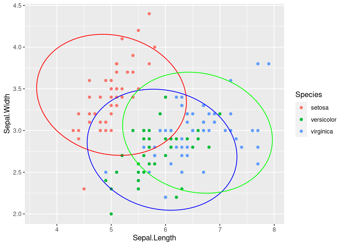
Figure 1.11: Iris dataset with different shapes for test and training and different colours for each class
Using linear discriminant analysis, we can classify the iris flowers into one of the three classes based on the four features.
# Linear discriminant analysis
library(MASS)
lda_results <- lda(Species ~ Sepal.Length + Sepal.Width,
                   data = iris)
lda_results
## Call:
## lda(Species ~ Sepal.Length + Sepal.Width, data = iris)
##
## Prior probabilities of groups:
## setosa versicolor virginica
## 0.3333333 0.3333333 0.3333333
##
## Group means:
## Sepal.Length Sepal.Width
## setosa 5.006 3.428
## versicolor 5.936 2.770
## virginica 6.588 2.974
##
## Coefficients of linear discriminants:
## LD1 LD2
## Sepal.Length -2.141178 -0.8152721
## Sepal.Width 2.768109 -2.0960764
##
## Proportion of trace:
## LD1 LD2
## 0.9628 0.0372The coefficients of the linear discriminant function give us the coefficients of the linear combination of the variables that maximises the ratio of the between-class variance to the within-class variance. Essentially, the data points are being projected into a lower-dimensional space where the classes are well separated.
Figure 1.12: LDA results for the Iris dataset with ellipses representing the covariance for each class
Figure 1.13: LDA results for the Iris dataset with ellipses representing the pooled covariance utilised
# Plot the predicted classes by changing the shapes of the points
Predicted <- predict(lda_results)$class
ggplot(data = iris) +
  geom_point(aes(x = Sepal.Length, y = Sepal.Width, color = Species,
                 shape = Predicted))
Figure 1.14: LDA results for the Iris dataset with respect to the discriminant boundaries
Figure 1.15: LDA results for the Iris dataset with respect to the discriminant boundaries via klaR