Chapter 6 Model Interpretation
A general criticism of machine learning methods is that they are often black boxes: it is difficult to disentangle the influence of one variable from another. This is particularly true for complex models such as random forests and gradient boosting machines where very many simple models have been averaged or aggregated. However, there are several methods that can be used to interpret the results of these models.
There are several mechanistic insights that we may want to have given a set of data and a model:
Variable importance: Which variables are most important in predicting the outcome?
Variable interactions: Are there interactions between variables that are important in predicting the outcome?
Local interpretability: Given a single observation, can we understand why the model made the prediction it did?
Model structure: What does the model look like? What are the decision rules that the model is using?
In this chapter, we will explore several methods for interpreting the results of a model. We will use the DALEX package to do this. This package provides a unified interface for interpreting the results of a wide variety of models (akin to caret for cross-validation).
6.1 Variable importance
In a simple linear regression model, the coefficients of the model give us a direct measure of the importance of each variable. For example, consider the following linear regression model:
##
## Call:
## lm(formula = mpg ~ ., data = mtcars)
##
## Residuals:
##     Min      1Q  Median      3Q     Max
## -3.4506 -1.6044 -0.1196  1.2193  4.6271
##
## Coefficients:
##             Estimate Std. Error t value Pr(>|t|)
## (Intercept) 12.30337   18.71788   0.657   0.5181
## cyl         -0.11144    1.04502  -0.107   0.9161
## disp         0.01334    0.01786   0.747   0.4635
## hp          -0.02148    0.02177  -0.987   0.3350
## drat         0.78711    1.63537   0.481   0.6353
## wt          -3.71530    1.89441  -1.961   0.0633 .
## qsec         0.82104    0.73084   1.123   0.2739
## vs           0.31776    2.10451   0.151   0.8814
## am           2.52023    2.05665   1.225   0.2340
## gear         0.65541    1.49326   0.439   0.6652
## carb        -0.19942    0.82875  -0.241   0.8122
## ---
## Signif. codes:  0 '***' 0.001 '**' 0.01 '*' 0.05 '.' 0.1 ' ' 1
##
## Residual standard error: 2.65 on 21 degrees of freedom
## Multiple R-squared:  0.869,  Adjusted R-squared:  0.8066
## F-statistic: 13.93 on 10 and 21 DF,  p-value: 3.793e-07
The coefficients of the model give us a direct measure of the importance of each variable. For example, the coefficient of wt is -3.72, which means that for every one unit increase in wt, the predicted value of mpg decreases by 3.72.
It is also straight forward to determine the strength of interactions between variables.
##
## Call:
## lm(formula = mpg ~ . + cyl:disp, data = mtcars)
##
## Residuals:
##     Min      1Q  Median      3Q     Max
## -3.1697 -1.6096 -0.1275  1.1873  3.8355
##
## Coefficients:
##              Estimate Std. Error t value Pr(>|t|)
## (Intercept) 29.976395  18.535141   1.617   0.1215
## cyl         -1.789619   1.183617  -1.512   0.1462
## disp        -0.095947   0.049001  -1.958   0.0643 .
## hp          -0.033409   0.020359  -1.641   0.1164
## drat        -0.541227   1.584761  -0.342   0.7363
## wt          -3.552721   1.717760  -2.068   0.0518 .
## qsec         0.698111   0.664203   1.051   0.3058
## vs           0.828745   1.918957   0.432   0.6705
## am           0.819051   1.997640   0.410   0.6862
## gear         1.554511   1.405425   1.106   0.2818
## carb         0.144212   0.764824   0.189   0.8523
## cyl:disp     0.013762   0.005825   2.363   0.0284 *
## ---
## Signif. codes:  0 '***' 0.001 '**' 0.01 '*' 0.05 '.' 0.1 ' ' 1
##
## Residual standard error: 2.401 on 20 degrees of freedom
## Multiple R-squared:  0.8976, Adjusted R-squared:  0.8413
## F-statistic: 15.94 on 11 and 20 DF,  p-value: 1.441e-07
For example, the coefficient of cyl:disp is 0.01, which means that for every simultaneous unit increase in cyl and disp, the predicted value of mpg increases by 0.01.
6.1.1 Decision tree structure
Another method for interpreting the results of a model is to examine the decision tree structure of the model. Of course, decision trees are far more accessible than other ML methods. As we have seen, there are several packages in R that can be used to visualise the decision tree structure of a model.
In a random forest setting, the decision tree structure of the model can be used to determine the importance of each variable. The importance of each variable is determined by the number of times the variable is used in the decision tree structure.
Example
Here we will use the rpart package to visualise the decision tree structure of a random forest model.
library(randomForest)

# Fit the random forest model
rf_model <- randomForest(mpg ~ .,
                         data = mtcars)

# Extract the decision tree structure of the model
tree <- getTree(rf_model, k = 1, labelVar = TRUE)

# Examine the decision tree structure
tree
## left daughter right daughter split var split point status prediction
## 1 2 3 disp 163.8000 -3 20.02188
## 2 4 5 wt 2.3025 -3 24.08750
## 3 6 7 hp 197.5000 -3 15.95625
## 4 0 0 <NA> 0.0000 -1 29.52000
## 5 8 9 wt 3.0125 -3 21.61818
## 6 10 11 vs 0.5000 -3 16.96364
## 7 0 0 <NA> 0.0000 -1 13.74000
## 8 12 13 drat 3.6600 -3 21.17778
## 9 0 0 <NA> 0.0000 -1 23.60000
## 10 14 15 wt 3.8125 -3 16.21667
## 11 0 0 <NA> 0.0000 -1 17.86000
## 12 0 0 <NA> 0.0000 -1 19.70000
## 13 16 17 vs 0.5000 -3 21.36250
## 14 0 0 <NA> 0.0000 -1 15.62000
## 15 0 0 <NA> 0.0000 -1 19.20000
## 16 0 0 <NA> 0.0000 -1 21.00000
## 17 18 19 carb 1.5000 -3 21.48333
## 18 0 0 <NA> 0.0000 -1 21.50000
## 19 0 0 <NA> 0.0000 -1 21.40000A function called importance within the randomForest package can be used to identify “important” variables. The measure of importance is the total decrease in node impurities from splitting on the variable, averaged over all trees. For classification, the node impurity is measured by the Gini index. For regression, it is measured by residual sum of squares.
##      IncNodePurity
## cyl      182.17791
## disp     234.43997
## hp       186.51583
## drat      70.92559
## wt       261.43699
## qsec      32.46751
## vs        27.20834
## am        18.79644
## gear      18.72446
## carb      27.88301
Looking at this measure alone, cyl, disp, hp and wt stand out as the most important as they are allowing the tree algorithm to split into relatively purer branches.
For a random forest model, we can also count how many times variables are used in the decision tree structure.
# Count how many times variables are used in the
# decision tree structure
variable.names(mtcars)[-1]
## [1] "cyl" "disp" "hp" "drat" "wt" "qsec" "vs" "am" "gear" "carb"## [1] 317 841 788 502 777 510 136 103 181 354This might suggest that disp is the most important variable in the model, but it could be that am is the most important but its influence is captured early in the decision tree structure.
Instead, we might count the number of times each variable is used for the first split in a decision tree within the random forest:
# Count how many times each variable is used for the
# first split in a decision tree
first.split <- sapply(1:rf_model$ntree, function(i) {
  rfTree <- getTree(rf_model, k = i, labelVar = TRUE)[1,3]
  variable.names(mtcars)[-1][rfTree]
})

table(first.split)
## first.split
## am cyl disp drat hp qsec vs wt
## 4 92 99 77 87 47 24 70Now, as the first division tends to be the most important in terms of predicting the outcome, we can see that disp and cyl seem to be the most important variables in the model.
6.1.2 Permutation-based variable importance
One way to determine the importance of each variable in a random forest or gradient boosting machine is to use a permutation-based variable importance method. This method works as follows:
Fit the model to the data.
For each variable in turn,
- randomly permute the values of that variable in the data;
- calculate the change in the model’s performance.
- The importance of each variable is the average change in the model’s performance across all permutations.
If a variable is important in predicting the outcome, then permuting the values of that variable should result in a large change in the model’s performance. Conversely, if a variable is not important in predicting the outcome, then permuting the values of that variable should result in a small change in the model’s performance.
The algorithm briefly outlined here is a one-at-a-time method. It is possible that such a method may miss important interactions between variables. There are other methods that can be used to determine the importance of interactions between variables.
Example
Here we will look at this strategy for a linear regression model and consider its utility in contrast to the more traditional hypothesis tests. Again, instead of relying on a package, we will implement this method ourselves.
# Fit the model
lm_model <- lm(mpg ~ ., data = mtcars)

# Hypothesis test results for each variable
summary(lm_model)
##
## Call:
## lm(formula = mpg ~ ., data = mtcars)
##
## Residuals:
## Min 1Q Median 3Q Max
## -3.4506 -1.6044 -0.1196 1.2193 4.6271
##
## Coefficients:
## Estimate Std. Error t value Pr(>|t|)
## (Intercept) 12.30337 18.71788 0.657 0.5181
## cyl -0.11144 1.04502 -0.107 0.9161
## disp 0.01334 0.01786 0.747 0.4635
## hp -0.02148 0.02177 -0.987 0.3350
## drat 0.78711 1.63537 0.481 0.6353
## wt -3.71530 1.89441 -1.961 0.0633 .
## qsec 0.82104 0.73084 1.123 0.2739
## vs 0.31776 2.10451 0.151 0.8814
## am 2.52023 2.05665 1.225 0.2340
## gear 0.65541 1.49326 0.439 0.6652
## carb -0.19942 0.82875 -0.241 0.8122
## ---
## Signif. codes: 0 '***' 0.001 '**' 0.01 '*' 0.05 '.' 0.1 ' ' 1
##
## Residual standard error: 2.65 on 21 degrees of freedom
## Multiple R-squared: 0.869, Adjusted R-squared: 0.8066
## F-statistic: 13.93 on 10 and 21 DF, p-value: 3.793e-07# Calculate the performance of the model
performance <- summary(lm_model)$r.squared
# Permute the values of each variable in turn
permuted_performance <- sapply(names(mtcars[,-1]),
function(var) {
# Permute the values of the variable
permuted_data <- mtcars
permuted_data[[var]] <- sample(permuted_data[[var]])
# Fit the model to the permuted data
permuted_lm_model <- lm(mpg ~ ., data = permuted_data)
# Calculate the performance of the model
permuted_performance <- summary(permuted_lm_model)$r.squared
# Return the change in performance
return(performance - permuted_performance)
})
# Plot the results
barplot(permuted_performance,
names.arg = names(mtcars[,-1]),
las = 2)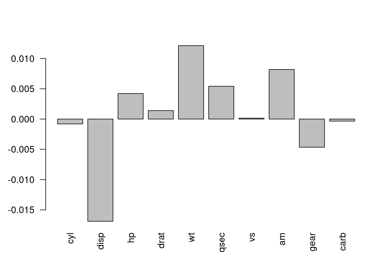
Figure 6.1: The change in performance of the model when the values of each variable are permuted.
There are, of course, packages available in R that will implement this method for you. One such package is DALEX.
Example
Now, we will utilise the DALEX package to determine the importance of each variable in a random forest model for the Boston housing data.
##
## Attaching package: 'ISLR2'
## The following object is masked from 'package:MASS':
##
## Boston## Registered S3 method overwritten by 'DALEX':
## method from
## print.description questionr## Welcome to DALEX (version: 2.4.3).
## Find examples and detailed introduction at: http://ema.drwhy.ai/
## Additional features will be available after installation of: ggpubr.
## Use 'install_dependencies()' to get all suggested dependencies# Fit the random forest model
rf_model <- randomForest(medv ~ ., data = Boston)
# Create an explainer object
explainer <- explain(rf_model,
data = Boston[-14],
y = Boston$medv)## Preparation of a new explainer is initiated
## -> model label : randomForest ( default )
## -> data : 506 rows 13 cols
## -> target variable : 506 values
## -> predict function : yhat.randomForest will be used ( default )
## -> predicted values : No value for predict function target column. ( default )
## -> model_info : package randomForest , ver. 4.7.1.1 , task regression ( default )
## -> predicted values : numerical, min = 6.821549 , mean = 22.52383 , max = 48.78306
## -> residual function : difference between y and yhat ( default )
## -> residuals : numerical, min = -5.040081 , mean = 0.008971517 , max = 9.705796
## A new explainer has been created!# Calculate the importance of each variable
variable_importance <- variable_importance(explainer)
variable_importance## variable mean_dropout_loss label
## 1 _full_model_ 1.425553 randomForest
## 2 medv 1.425553 randomForest
## 3 zn 1.474409 randomForest
## 4 chas 1.497513 randomForest
## 5 rad 1.574467 randomForest
## 6 age 1.868436 randomForest
## 7 tax 1.963858 randomForest
## 8 indus 2.079444 randomForest
## 9 ptratio 2.329765 randomForest
## 10 crim 2.408515 randomForest
## 11 dis 2.586561 randomForest
## 12 nox 2.630679 randomForest
## 13 rm 5.313940 randomForest
## 14 lstat 6.596881 randomForest
## 15 _baseline_ 12.637616 randomForestHere, mean_dropout_loss is the average change in the model’s performance across all permutations. The larger the value, the more important the variable is in predicting the outcome.
6.2 Main effect visualisations
6.2.1 Main effects
A main effect is the effect of a variable on the outcome, while holding all other variables constant. To help us to understand the utility of these let’s consider a situation where we know the true model generating the data.
Example
Here, we have one outcome variable and two explanatory variables. The true model is:
\[ Y = X_1 + X_2^2. \] We will have strongly correlated explanatory variables:
\[\begin{align*} X_1 &\sim \text{Uni}(0, 1), \\ X_2 &= X_1 + \epsilon, \quad \epsilon \sim \text{N}(0, 0.02). \end{align*}\]
Here’s some data for us to work with:
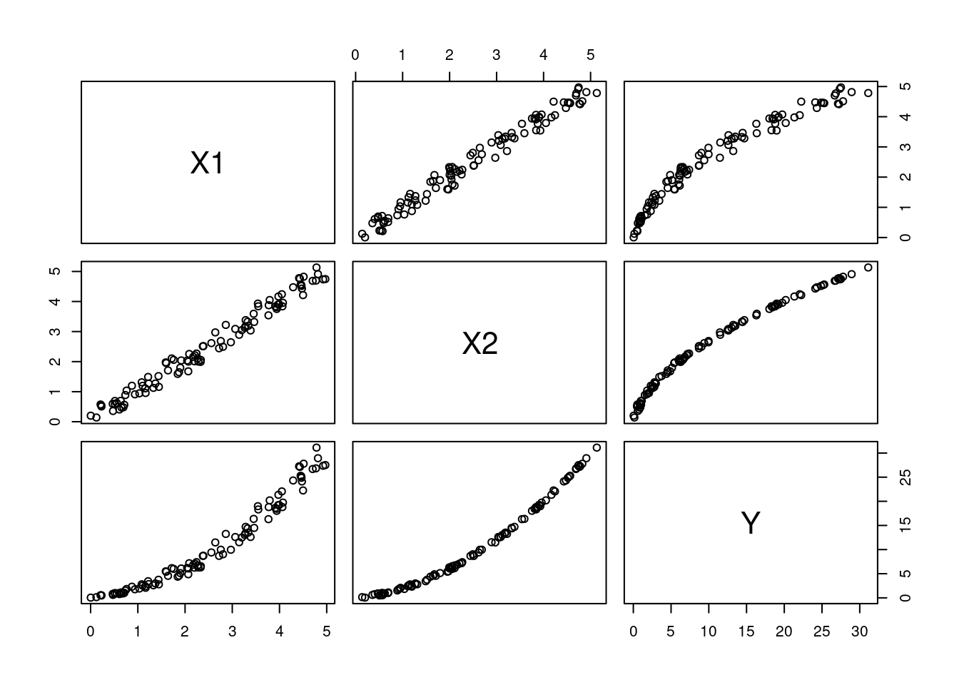
Figure 6.2: The relationship between the variables in the data.
It is trivial to derive the main effect of the model for fixed values of \(X_1\): \[ \begin{aligned} \text{E}[Y|X_1=x_1] &= x_1 + \text{E}[X_2^2|X_1=x_1] \\ &= x_1 + \text{E}[(x_1 + \epsilon)^2]\\ &= x_1 + x_1^2 + \text{E}[\epsilon^2]. \end{aligned} \]
Similarly for fixed values of \(X_2\): \[ \begin{aligned} \text{E}[Y|X_2=x_2] &= \text{E}[X_1|X_2=x_2] + x_2^2 \\&= \text{E}[x_2 - \epsilon] + x_2^2 \\&= x_2 + x_2^2. \end{aligned} \] You will notice in these derivations that we have had to account for the joint distribution of the variables.
Figures 6.3 and 6.4 show the main effects of \(X_1\) and \(X_2\) on \(Y\) respectively (plotted against all the observations).
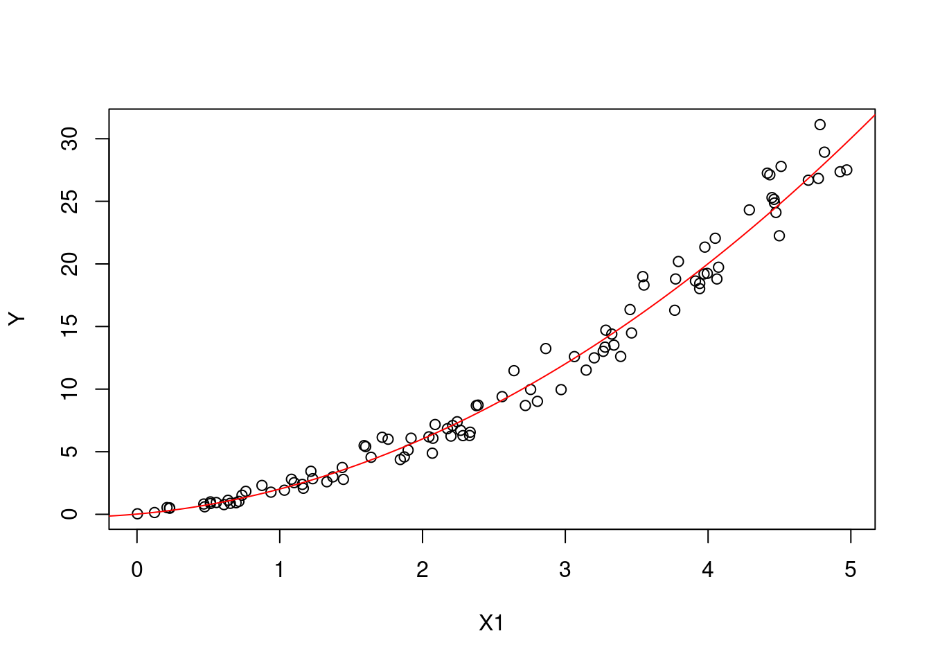
Figure 6.3: The main effect of X1 on Y.
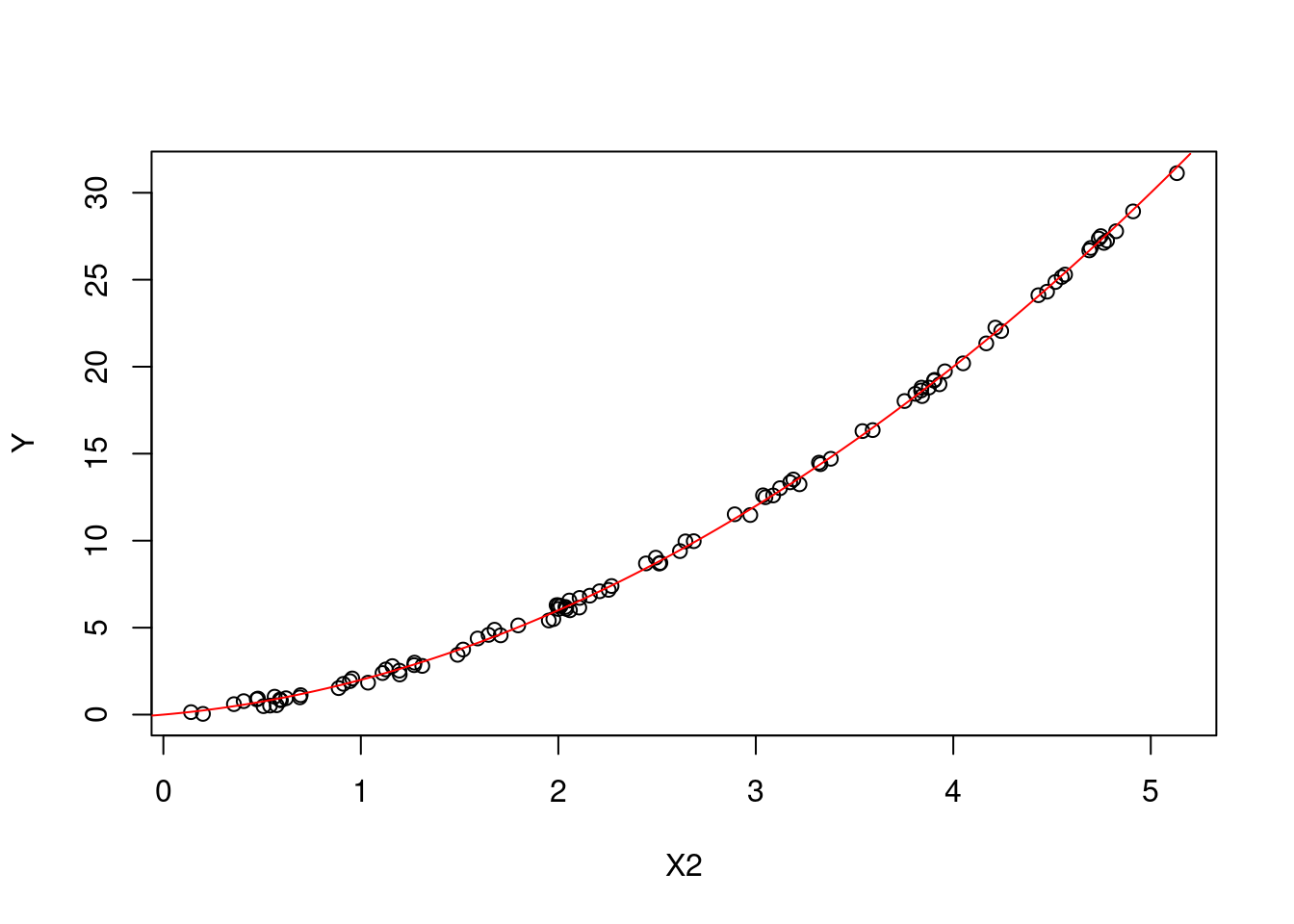
Figure 6.4: The main effect of X2 on Y.
6.2.2 Partial dependence plots
One method for interpreting the results of a model is to use partial dependence plots. A partial dependence plot shows the relationship between a variable and the outcome, while holding all other variables constant. This allows us to see the effect of a variable on the outcome, while controlling for the effects of other variables.
Example
Here, we will use the iml package to create a partial dependence plot for the random forest model for the Boston data.
library(iml)

# Create an explainer object
explainer <- Predictor$new(rf_model,
                           data = Boston)

# Create a partial dependence plot for the variable `lstat`
lstat_pd <- FeatureEffect$new(explainer,
                              feature = "lstat",
                              method = 'pdp')

# Plot the partial dependence plot
plot(lstat_pd)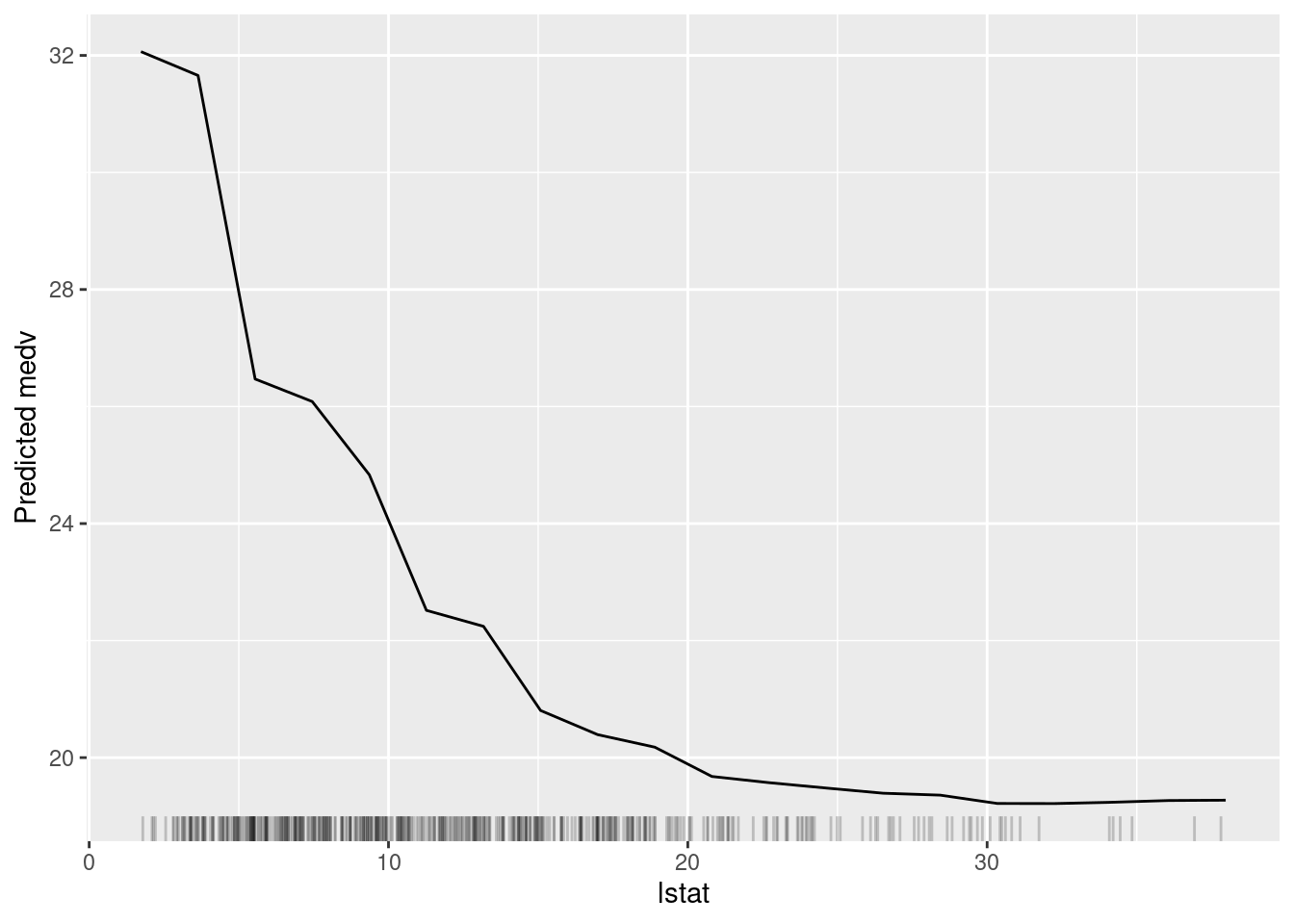
Figure 6.5: The partial dependence plot for the variable lstat.
In Figure 6.5, we can see a clear negative relationship between lstat and medv. As lstat increases, medv decreases. This is consistent with our understanding of the data because lstat is the percentage of lower status of the population, which is likely to be negatively correlated with the median value of owner-occupied homes.
6.2.3 Accumulated local effects
Another method for interpreting the results of a model is to use accumulated local effects. Accumulated local effects focus on the difference in predictions when a variable is changed, rather than the average prediction itself. We calculate them in the following way:
- Partitioning the variable’s range:
- Divide the range of the variable into a reasonable number of intervals;
- The number of intervals can influence the smoothness of the ALE plot;
- For each interval, calculate the average value of the variable within that interval.
- Calculating Local Effects:
- For each interval, calculate the difference in the average model prediction between:
- The original data within that interval;
- The data where the variable values within that interval are shifted by a small amount (e.g., half the interval width);
- This difference represents the local effect of the variable within that interval.
- Accumulating Local Effects:
- Start with the lowest interval and calculate the local effect for that interval;
- For each subsequent interval, add the local effect of that interval to the accumulated effect from the previous intervals;
- This gives you the cumulative effect of the variable on the model’s predictions up to that point.
Example
Here, we will again use the iml package to create an ALE plot.
lstat_pd <- FeatureEffect$new(explainer,
                              feature = "lstat",
                              method = 'ale')

# Plot the partial dependence plot
plot(lstat_pd)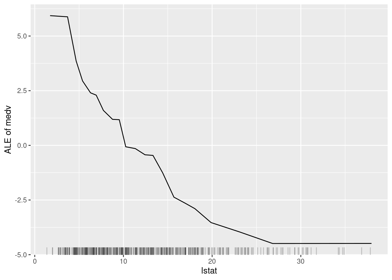
Figure 6.6: The ALE plot for the variable lstat.
Figure 6.6 is very similar to Figure 6.5. This is perhaps because there is not a great amount of interaction between lstat and the other variables in the model. However, the ALE plot is more interpretable than the partial dependence plot because it shows the difference in predictions when lstat is changed, rather than the average prediction itself.