Topic 5 - Functions of Several Variables

5.0 Introduction

In our previous studies (at school and in the previous Topics) we’ve learnt about calculus of functions of a single variable. Life isn’t usually that simple, and many useful physical quantities depend on several independent parameters.

For instance, in Physics we have the ideal gas law which links the pressure $P$ of a hypothetical ideal gas in terms of other quantities: \[P=\frac{nRT}{V}\] where $V$ is the volume of the gas, $T$ is the absolute temperature, $n$ is the amount of substance and $R$ is the ideal gas constant (all measured in suitable units).

We can ask: how does the pressure vary for a fixed amount of gas when $T$ varies. Or when $V$ varies. Or when both $T$ and $V$ vary in some way.

In this Topic, we’ll discuss partial differentiation of functions of several variables, which generalises the notion of the derivative to higher dimensions, and we’ll see how this helps to analyse their behaviour.

One can also consider integration of multi-variable functions. One of the many applications of this is calculating volumes under surfaces in the same way ordinary integration gives areas under curves.

We won’t discuss integration in this short Topic (leaving it to other modules you may study) but we will look at various other problems involving surfaces such as finding tangent planes, maxima and minima.

5.1 Partial Differentiation

We’ll begin with a simple geometric example illustrating the general idea. Consider a cone with base circle of radius $r$ and height $h.$ Its volume depends on both $r$ and $h$.

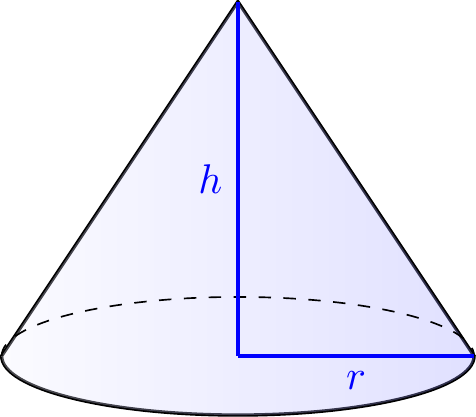
In particular, we know that this cone has volume $V(r,h)=\dfrac{1}{3}\pi r^2h$.

If $h$ remains constant but $r$ changes, what is the rate of change of $V$ with respect to $r$?

Although $V(r,h)$ is a function of two variables, keeping $h$ constant means it only depends on how $r$ varies. The rate of change is obtained by just differentiating with respect to $r$. We write \[ \frac{\partial V}{\partial r}=\frac{2}{3}\pi rh. \] This is the idea of partial differentiation. Note that we use the “curly d” symbol $\partial$ rather than a normal $d$. This conventional notation is used to remind us that we are only letting $r$ vary.

Similarly, we can ask about the rate of change of $V$ when $r$ is fixed and $h$ changes: \[ \frac{\partial V}{\partial h}=\frac{1}{3}\pi r^2. \]

Given a function of several variables, $f(x,y,z,...)$, the partial derivative of $f$ with respect to $x$ is obtained by treating all variables in the formula for $f$ except $x$ as constants, and differentiating with respect to $x$. We write this partial derivative as \[\frac{\partial f}{\partial x}.\] Similarly, there are partial derivatives $\dfrac{\partial f}{\partial y}$, $\dfrac{\partial f}{\partial z}$,… for the other variables.

Example. $\,$ Suppose we are given $f(x,y,z)=e^{y^2}\cos(xyz)$.

(This could be giving values of a useful quantity, e.g temperature, electric charge, density,… in terms of the position $(x,y,z)$ in 3-dimensional space.)

If $y$ and $z$ stay fixed, find the rate of change of $f$ with respect to $x$.

As above, we treat $y$ and $z$ as constants and just differentiate with respect to $x$. We get \[ \frac{\partial f}{\partial x}=-yze^{y^2}\sin(xyz). \] Similarly, (applying the product and chain rules) we find \[\frac{\partial f}{\partial y}=2ye^{y^2}\cos(xyz)-xze^{y^2}\sin(xyz)\] and \[\frac{\partial f}{\partial z}=-xye^{y^2}\sin(xyz). \]

We can also differentiate multiple times to obtain higher derivatives such as \[ \dfrac{\partial^2 f}{\partial x^2}= \dfrac{\partial}{\partial x}\left(\dfrac{\partial f}{\partial x}\right), \qquad \dfrac{\partial^2 f}{\partial y^2}= \dfrac{\partial}{\partial y}\left(\dfrac{\partial f}{\partial y}\right),... \] Now that we have multiple variables, however, we can also mix the derivatives to get \[ \dfrac{\partial^2 f}{\partial x\partial y}= \dfrac{\partial}{\partial x}\left(\dfrac{\partial f}{\partial y}\right), \qquad \dfrac{\partial^2 f}{\partial y\partial x}= \dfrac{\partial}{\partial y}\left(\dfrac{\partial f}{\partial x}\right),... \]

Example. $\,$ Let $f(x,y)=\cos y + \sin(xy)$. Then \[\begin{align*} \frac{\partial f}{\partial x}&=y\cos(xy) \\ \frac{\partial f}{\partial y}&=-\sin y+x\cos(xy). \end{align*}\] Also \[\begin{align*} \frac{\partial^2 f}{\partial x^2}&= \frac{\partial}{\partial x}\Big(y\cos(xy)\Big) =-y^2\sin(xy), \\ \frac{\partial^2 f}{\partial y^2} &=\frac{\partial}{\partial y}\Big(-\sin y+x\cos(xy)\Big) =-\cos y-x^2\sin(xy). \end{align*}\]

We can also find mixed derivatives. In this case, these are \[\frac{\partial^2 f}{\partial y\partial x} =\frac{\partial}{\partial y}\left(\frac{\partial f}{\partial x}\right) =\cos(xy)-xy\sin(xy)\] and \[\frac{\partial^2 f}{\partial x\partial y} =\frac{\partial}{\partial x}\left(\frac{\partial f}{\partial y}\right) =\cos(xy)-xy\sin(xy).\]

Notice these mixed derivatives are equal. This happens for all “reasonably nice functions” (in particular, all of the functions we’ll meet in the Topic) and one can usually assume \[\frac{\partial^2 f}{\partial y\partial x} =\frac{\partial^2 f}{\partial x\partial y}.\]

Actually, one has to go out of one’s way to construct examples where this symmetry is broken. Strange-looking functions such as \[f(x,y)=\begin{cases} \dfrac{xy(x^2-y^2)}{x^2+y^2} & \text{for $(x,y)\neq (0,0)$,}\\ 0 & \text{for $(x,y)=(0,0),$} \end{cases}\] which has nasty behaviour at the origin is one such example (but this is beyond our course!)

5.2 The Chain Rule

Recall the Chain Rule for functions of one variable: if $f(x)$ is a function of $x$ and if $x$ is a function $x(t)$ of $t$, then \[\frac{df}{dt}=\frac{df}{dx}\,\frac{dx}{dt}.\] There is an extension of this to our new multi-variable world. For a function of two variables $f(x,y)$ where $x=x(t),\, y=y(t)$, we have \[ \frac{df}{dt}=\frac{\partial f}{\partial x}\,\frac{dx}{dt}+ \frac{\partial f}{\partial y}\,\frac{dy}{dt}.\] The idea here is $f$ is depending on $t$ through both $x$ and $y$ “partially” and the two terms contribute to give the total variation. A similar formula is true with more variables, e.g. for $f(x,y,z)$, \[ \frac{df}{dt}=\frac{\partial f}{\partial x}\,\frac{dx}{dt}+ \frac{\partial f}{\partial y}\,\frac{dy}{dt}+ \frac{\partial f}{\partial z}\,\frac{dz}{dt}. \]

Let’s see how this works using the cone example from the last section:

Example. $\,$ Suppose a cone has height $h(t)$, base circle of radius $r(t)$ which vary with time $t$ in the following way: \[r(t)=2+\sin{t}\qquad\text{and}\qquad h(t)=2+\cos{t}.\] What is the rate of change of the volume $V=\dfrac{1}{3}\pi r^2h$ with respect to time?

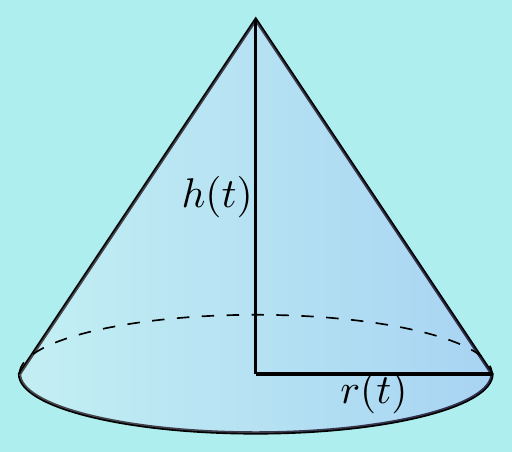
We will answer this in two ways.

Method 1.$\;$ Substitute $h(t)$ and $r(t)$ into the expression for $V$ and differentiate this directly with respect to $t$. \[\begin{align*} V(r,h)&=\frac{1}{3}\pi r^2h\ \\ \implies V(t)&=\frac{1}{3}\pi \left(2+\sin t\right)^2\left(2+\cos t\right)\ \\ \implies \frac{dV}{dt} &=\frac{1}{3}\pi\left(2\cos t\left(2+\sin t\right)\left(2+\cos t\right) -\left(2+\sin t\right)^2\sin t\right). \end{align*}\]

Method 2.$\;$ Using the Chain Rule given above \[\begin{align*} \frac{dV}{dt}&=\frac{\partial V}{\partial r}\frac{dr}{dt}+ \frac{\partial V}{\partial h}\frac{dh}{dt} \\ &=\frac{2}{3}\pi rh\cos t-\frac{1}{3}\pi r^2\sin t \\ &=\frac{2}{3}\pi\left(2+\sin t\right)\left(2+\cos t\right)\cos t -\frac{1}{3}\pi \left(2+\sin t\right)^2\sin t \end{align*}\] which is the same expression as in Method 1.

There is also a Chain Rule of the following form: for $f(x,y)$ where $x=x(u,v),\, y=y(u,v)$, we have \[\begin{align*} \frac{\partial f}{ \partial u}= \frac{\partial f}{ \partial x}\frac{\partial x}{ \partial u}+ \frac{\partial f}{ \partial y}\frac{\partial y}{ \partial u} \quad\text{and}\quad \frac{\partial f}{ \partial v}= \frac{\partial f}{ \partial x}\frac{\partial x}{ \partial v}+ \frac{\partial f}{ \partial y}\frac{\partial y}{ \partial v}. \end{align*}\]

Example. $\,$ Suppose $f(x,y)=\sin(xy)$ where $x=2u+2v$ and $y=2u-2v$.

Then we can evaluate $\dfrac{\partial f}{ \partial u}$ and $\dfrac{\partial f}{ \partial v}$ in two ways as in the previous example.

Method 1.$\;$ Substitute the values of $x$ and $y$ into the expression for $f$ to give
\[\begin{align*} f(x,y)&=\sin(xy) \\ &=\sin\left(4\left(u+v\right)\left(u-v\right)\right) \\ &=\sin\left(4\left(u^2-v^2\right)\right) \end{align*}\] and so differentiating gives \[\frac{\partial f}{ \partial u}=8u\cos\left(4\left(u^2-v^2\right)\right) \qquad \text{and} \qquad \frac{\partial f}{ \partial v}=-8v\cos\left(4\left(u^2-v^2\right)\right). \]

Method 2.$\;$ Using the Chain Rule given above \[\begin{align*} \frac{\partial f}{ \partial u}&= \frac{\partial f}{ \partial x}\frac{\partial x}{ \partial u}+ \frac{\partial f}{ \partial y}\frac{\partial y}{ \partial u} \\ &=2y\cos(xy)+2x\cos(xy) \\ &=2\left(2u-2v+2u+2v\right)\cos\left(4\left(u^2-v^2\right)\right) \\ &=8u\cos\left(4\left(u^2-v^2\right)\right) \end{align*}\] and similarly, \[\begin{align*} \frac{\partial f}{ \partial v}&= \frac{\partial f}{ \partial x}\frac{\partial x}{ \partial v}+ \frac{\partial f}{ \partial y}\frac{\partial y}{ \partial v} \\ &=2y\cos(xy)-2x\cos(xy) \\ &=2\left(2u-2v-(2u+2v)\right)\cos\left(4\left(u^2-v^2\right)\right) \\ &=-8v\cos\left(4\left(u^2-v^2\right)\right)\notag \end{align*}\] which are the same expressions as in Method 1.

5.3 Changes of variables

Just like in usual single variable calculus, changing variables is important in our new multi-variable situation, though as one would expect, things get more complicated.

Example. $\,$ Suppose that $f(x,y)$ is a function of $x,y$ where $x=ve^u$ and $y=ve^{-u}$. Rewrite $\dfrac{\partial f}{\partial u}$ and $v\dfrac{\partial f}{\partial v}$ in terms of $x$ and $y$ and derivatives with respect to $x$ and $y$.

First calculate $\hspace{2cm}\dfrac{\partial x}{\partial u}=ve^u=x$, $\hspace{1cm}\dfrac{\partial y}{\partial u}=-ve^{-u}=-y$,

and

$\hspace{3.95cm}\dfrac{\partial x}{\partial v}=e^u=\dfrac{x}{v}$, $\hspace{1.1cm}\dfrac{\partial y}{\partial v}=e^{-u}=\dfrac{y}{v}.$

Applying the chain rule then gives \[\begin{align*} \frac{\partial f}{\partial u} =\frac{\partial x}{\partial u}\frac{\partial f}{\partial x}+ \frac{\partial y}{\partial u}\frac{\partial f}{\partial y} &=x\frac{\partial f}{\partial x}-y\frac{\partial f}{\partial y}\tag{$\star$} \end{align*}\] and
\[\begin{align*} v\frac{\partial f}{\partial v} =v\left[\frac{\partial x}{\partial v}\frac{\partial f}{\partial x}+ \frac{\partial y}{\partial v}\frac{\partial f}{\partial y}\right] &=x\frac{\partial f}{\partial x}+ y\frac{\partial f}{\partial y}.\tag{$\star\star$} \end{align*}\]

Handling second derivatives is much more difficult and requires a lot of care. Here’s a tricky example (harder than anything you’d get on an exam!) to indicate what’s going on.

Example. $\,$ Let’s consider some 2nd derivatives of the same functions as the last example and find a formula for \[v\frac{\partial^2 f}{\partial u\partial v}-\frac{\partial f}{\partial u}\] in terms of derivatives with respect to $x$ and $y$.

First, use ($\star$), ($\star\star$) and the product rule to see \[\begin{align*} v\frac{\partial^2 f}{\partial u\partial v} =\frac{\partial}{\partial u}\left(v\frac{\partial f}{\partial v}\right) &=\frac{\partial}{\partial u} \left(x\frac{\partial f}{\partial x}+y\frac{\partial f}{\partial y}\right) \\ &=\frac{\partial x}{\partial u}\frac{\partial f}{\partial x} +x\frac{\partial}{\partial u}\left(\frac{\partial f}{\partial x}\right) +\frac{\partial y}{\partial u}\frac{\partial f}{\partial y} +y\frac{\partial}{\partial u}\left(\frac{\partial f}{\partial y}\right) \\ &=x\frac{\partial f}{\partial x} +x\frac{\partial}{\partial u}\left(\frac{\partial f}{\partial x}\right) -y\frac{\partial f}{\partial y} +y\frac{\partial}{\partial u}\left(\frac{\partial f}{\partial y}\right) \\ &=\frac{\partial f}{\partial u} +x\frac{\partial}{\partial u}\left(\frac{\partial f}{\partial x}\right) +y\frac{\partial}{\partial u}\left(\frac{\partial f}{\partial y}\right) \tag{$\star\star\star$} \end{align*}\]

We are left with the problem of finding $\dfrac{\partial}{\partial u}\left(\dfrac{\partial f}{\partial x}\right)$ and $\dfrac{\partial}{\partial u}\left(\dfrac{\partial f}{\partial y}\right)$.

However, notice ($\star$) and ($\star\star$) can apply to any function of $x$ and $y$, not just $f(x,y)$.

In particular, replacing $f$ by $\dfrac{\partial f}{\partial x}$ in ($\star$) gives \[\begin{align*} \frac{\partial}{\partial u}\left(\frac{\partial f}{\partial x}\right) &=x\frac{\partial}{\partial x}\left(\frac{\partial f}{\partial x} \right)- y\frac{\partial}{\partial y}\left(\frac{\partial f}{\partial x} \right) \\ &=x\frac{\partial^2 f}{\partial x^2}-y\frac{\partial^2 f}{\partial y\partial x}. \end{align*}\] Similarly, replacing $f$ by $\dfrac{\partial f}{\partial y}$ in ($\star$) gives \[\dfrac{\partial}{\partial u}\left(\dfrac{\partial f}{\partial y}\right) =x\dfrac{\partial^2 f}{\partial x\partial y}-y\dfrac{\partial^2 f}{\partial y^2}.\] Substituting these into ($\star\star\star$) gives \[\begin{align*} v\frac{\partial^2 f}{\partial u\partial v} &=\frac{\partial f}{\partial u} +x\left[x\frac{\partial^2 f}{\partial x^2}-y\frac{\partial^2 f}{\partial y\partial x}\right] +y\left[x\dfrac{\partial^2 f}{\partial x\partial y}-y\dfrac{\partial^2 f}{\partial y^2}\right] \end{align*}\] and so we finally obtain \[v\frac{\partial^2 f}{\partial u\partial v}-\frac{\partial f}{\partial u} =x^2\frac{\partial^2 f}{\partial x^2}-y^2\frac{\partial^2 f}{\partial y^2}.\]

These types of formulas may look cumbersome, but they can be very useful, for instance, in studying partial differential equations. Think of it as changing variables from $(x,y)$ to $(u,v)$ and expressing a particular differential “object” in the new variables. In the above (difficult!) example, we are essentially using \[\frac{\partial}{\partial u}=x\frac{\partial}{\partial x}-y\frac{\partial}{\partial y} \quad\text{and}\quad v\frac{\partial}{\partial v}=x\frac{\partial}{\partial x}+ y\frac{\partial}{\partial y}.\] As in single variable calculus, a well-chosen change of variables can make solving a problem much easier. (See the questions involving the Laplace equation in the Study Problems.)

A more familiar change of variables is polar coordinates where we convert using $x=r\cos\theta$ and $y=r\sin\theta$ and, given $x$ and $y$, we can find $r$ and $\theta$.

In particular, $\dfrac{\partial x}{\partial r}=\cos\theta$ and as $r=\sqrt{x^2+y^2}$, we have $\dfrac{\partial r}{\partial x}=\dfrac{x}{\sqrt{x^2+y^2}}=\dfrac{x}{r}=\cos\theta.$

Notice something strange has happened – we don’t have $\dfrac{\partial x}{\partial r}=\left(\dfrac{\partial r}{\partial x}\right)^{-1}$ as we might expect in single variable calculus. The reason is the partial derivative $\dfrac{\partial x}{\partial r}$ is keeping $\theta$ constant whereas $\dfrac{\partial r}{\partial x}$ is keeping $y$ constant and these are not equivalent. Occasionally (in some books and notes), people use notation such as \[\left(\dfrac{\partial x}{\partial r}\right)_\theta \quad\text{and}\quad \left(\dfrac{\partial r}{\partial x}\right)_y \] to keep track of which variables are being kept constant.

5.4 Directional derivatives and the gradient

We can think of a multi-variable function $f(x,y,z)$ as a function of a position vector – it is $f({\bf p})$ where ${\bf p}=(x,y,z)$. The same goes for the partial derivatives. Now, evaluating $\partial f/\partial x$ at ${\bf p}$ gives the rate of change of $f$ as we move from ${\bf p}$ in the direction parallel to the $x$-axis (since we are keeping $y$ and $z$ fixed). There are similar statements for the other derivatives $\partial f/\partial y$ and $\partial f/\partial z$. But what is the rate of change of $f$ in an arbitrary direction from a point?

Suppose we are given a point in $\mathbb{R}^3$ and a direction vector \[{\bf p}=\left(p_1,p_2,p_3\right)=p_1{\bf i}+p_2{\bf j}+p_3{\bf k}\] and \[{\bf v}=\left(v_1,v_2,v_3\right)=v_1{\bf i}+v_2{\bf j}+v_3{\bf k}. \]

Furthermore, for now, assume that $\bf v$ has unit length so that $|{\bf v}| = \sqrt{v_1^2+v_2^2+v_3^2}=1.$ From the first term, we know that the line through $\bf{p}$ and in direction $\bf{v}$ is given by \[{\bf r}(t)={\bf p}+t{\bf v}.\] Here, $t$ is a real parameter - if we think of this as time, then the point ${\bf r}(t)$ moves along the line starting at ${\bf p}={\bf r}(0)$ and at unit velocity ${\bf v}=\dfrac{d{\bf r}}{dt}$. In Cartesian coordinates, \[\begin{align*} {\bf r}(t)&=\left(x(t),y(t),z(t)\right) =\left(p_1+tv_1, p_2+tv_2,p_3+tv_3\right) \end{align*}\] so the rate of change of a function $f(x,y,z)$ along ${\bf r}(t)$ can be written as a scalar product: \[\begin{align*} \frac{df}{dt}&=\frac{\partial f}{\partial x}\frac{dx}{dt}+ \frac{\partial f}{\partial y}\frac{dy}{ dt}+ \frac{\partial f}{ \partial z}\frac{dz}{ dt} \\ &=\left(\frac{\partial f}{\partial x}, \frac{\partial f}{\partial y}, \frac{\partial f}{\partial z}\right)\cdot \left(\frac{dx}{dt},\frac{dy}{dt},\frac{dz}{dt} \right) \\ &=\left(\frac{\partial f}{\partial x}, \frac{\partial f}{\partial y}, \frac{\partial f}{\partial z}\right)\cdot \left(v_1,v_2,v_3 \right) =\left(\frac{\partial f}{\partial x}, \frac{\partial f}{ \partial y}, \frac{\partial f}{\partial z}\right)\cdot {\bf v} \end{align*}\]

This leads us to introduce the following concept.

Definition$\;$ The gradient of $f(x,y,z)$ is the vector-valued function \[\nabla f=\left(\frac{\partial f}{\partial x}, \frac{\partial f}{\partial y}, \frac{\partial f}{\partial z}\right) =\frac{\partial f}{\partial x}{\bf i}+\frac{\partial f}{\partial y}{\bf j}+ \frac{\partial f}{\partial z}{\bf k}. \]

(Note $\nabla f$ is also sometimes written ${\bf grad}\;f$.)

Thus, the rate of change of $f(x,y,z)$ at ${\bf p}$ in unit direction ${\bf v}$ is given by \[\left.\frac{df}{dt}\right|_{t=0} =\nabla f({\bf p})\cdot{\bf v}.\] If ${\bf v}$ is not a unit vector, then dividing by $|{\bf v}|$ gives the general formula:

Definition$\;$ The directional derivative of $f$ at ${\bf p}$ in the direction ${\bf v}$ is $\nabla f\left({\bf p}\right)\cdot \dfrac{{\bf v}}{ \left|{\bf v}\right|}$.

Example. $\,$ If $f(x,y,z)=x^3-xy^2-z$, find the directional derivative of $f$ at the point ${\bf p}=(1,1,0)$ in the direction ${\bf v}=2{\bf i}-3{\bf j}+6{\bf k}$.

We first need to calculate the gradient of $f$ at the point: \[\nabla f=\left(3x^2-y^2\right){\bf i}-2xy{\bf j}-{\bf k} \quad\implies\quad \nabla f(1,1,0)=2{\bf i}-2{\bf j}-{\bf k}.\] Hence the required directional derivative is \[\left(2{\bf i}-2{\bf j}-{\bf k}\right)\cdot \left(2{\bf i}-3{\bf j}+6{\bf k}\right)\frac{1}{\sqrt{4+9+36}} =\frac{4+6-6}{\sqrt{49}}=\frac{4}{7}. \]

All of the above works in any number of dimensions. For instance, here’s a 2-d example:

Example. $\,$ The height of a slope above sea level is $f(x,y)=2y^2+x^2$ (in some unit of distance) at coordinates $(x,y)$. Find the rate of change of height (i.e. the rate of ascent) when starting at $(1,2)$ and moving at unit speed towards the south-east.

We need to calculate the directional derivative of $f$ at $(1,2)$ in the direction ${\bf i}-{\bf j}$. Now \[\nabla f =\left(\frac{\partial f}{\partial x},\frac{\partial f}{\partial y}\right) =\left(2x,4y\right) \quad\implies\quad \nabla f(1,2)=2{\bf i}+8{\bf j}.\] Hence the required directional derivative is \[ \left(2{\bf i}+8{\bf j}\right)\cdot\frac{\left({\bf i}-{\bf j}\right)}{\sqrt{1+1}} =-\frac{6}{\sqrt2}\]
and so the rate of change of height is $-6/\sqrt{2}\approx -4.24$.

Here is a natural question: given a function $f$ and a point ${\bf p}$, in which direction from ${\bf p}$ does $f$ have the largest directional derivative, and what is this largest value? For instance, in the previous example, in which direction is the steepest ascent, and how steep is it?

Recall that the directional derivative of $f$ at ${\bf p}$ in the direction ${\bf v}$ is \[\nabla f\left({\bf p}\right)\cdot \frac{{\bf v}}{\left|{\bf v}\right|} =\left|\nabla f\left({\bf p}\right)\right|\cos\theta\] where $\theta$ is the angle between $\nabla f\left({\bf p}\right)$ and ${\bf v}$. This clearly has maximum value when $\cos(\theta)=1$ so we need $\theta=0$ and hence ${\bf v}$ is parallel to $\nabla f({\bf p})$. Thus, the steepest increase is we move off in the direction $\nabla f({\bf p})$ and the maximum value is $\left|\nabla f({\bf p})\right|$.

Example. $\,$ If $f(x,y)=-\cos(xy)$, in what direction should one travel from $\left(\dfrac{\pi}{2},1\right)$ in order to maximise the rate of change of $f$?

We calculate $\nabla f(x,y)=\left(y\sin(xy),x\sin(xy)\right)$ and \[\nabla f\left(\frac{\pi}{2},1\right)={\bf i}+\frac{\pi}{2}{\bf j}. \] So we have to travel in the direction ${\bf i}+\frac{\pi}{2}{\bf j}$ and the maximum rate of change is \[\left|\nabla f\left(\frac{\pi}{2},1\right)\right|= \left|{\bf i}+\frac{\pi}{2}{\bf j}\right|=\sqrt{1+\frac{\pi^2}{4}}.\]

5.5 Tangent planes to surfaces

First, we give a brief reminder about planes and lines in 3-dimensional space and then look at some surfaces.

Note, in these applications it is often convenient to write vectors as rows rather than columns.

Planes.$\;$ The equation of the plane through the point ${\bf p}=(p_1,p_2,p_3)$ and normal to the vector ${\bf n}=n_1{\bf i}+n_2{\bf j}+n_3{\bf k}$ is given by \[\left({\bf x}-{\bf p}\right)\cdot {\bf n}=0.\] Putting in the coordinates ${\bf x}=(x,y,z)$, turns this into the familiar Cartesian form \[n_1x+n_2y+n_3z=C\] where $C=p_1n_1+p_2n_2+p_3n_3$. For example, the equation of the plane through $(2,-1,5)$ which is normal to $4{\bf i}+3{\bf j}-{\bf k}$ is \[4x+3y-z=4\times2+3(-1)-5=0.\]

Lines.$\;$ The equation of the line through ${\bf p}=(p_1,p_2,p_3)$ in the direction ${\bf v}=v_1{\bf i}+v_2{\bf j}+v_3{\bf k}$ is, in parametric form, given by \[{\bf x} = {\bf p} + t{\bf v}\] where $t$ is an arbitrary parameter. Putting in the coordinates ${\bf x}=(x,y,z)$ makes this \[\begin{align*} (x,y,z)&=(p_1,p_2,p_3)+t\left(v_1,v_2,v_3\right) \\ &=(p_1+tv_1,p_2+tv_2, p_3+tv_3). \end{align*}\] Rearranging by solving for $t$ gives the alternative Cartesian form: \[\lambda=\frac{x-p_1}{ v_1}=\frac{y-p_2}{ v_2}=\frac{z-p_3}{v_3}.\] For example, the equation of the line through $(2,-1,5)$ in the direction $4{\bf i}+3{\bf j}-{\bf k}$ is \[{\bf x}=(2,-1,5)+t\left(4,3,-1\right)\] or equivalently, in Cartesian form \[\frac{x-2}{4}=\frac{y+1}{3}=\frac{z-5}{-1}.\]

Surfaces.$\;$ We will consider surfaces with equations written in the form $f(x,y,z)=C$, where $C$ is a constant. These are the sometimes called level surfaces of the function $f$. Sometimes, it’s possible to rewrite these equations giving $z$ in terms of $x$ and $y$, but that won’t always be the case.

Examples. $\;$ You are probably familiar with a number of surfaces written in this form.

$(1)\;$ The sphere of radius $r$ and centred at the origin: \[f(x,y,z)=x^2+y^2+z^2=r^2\]

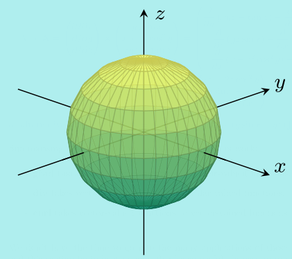
We could rewrite the equation as $z=\pm\sqrt{r^2-x^2-y^2}$ to get $0$, $1$ or $2$ possible values of $z$ for each choice of $x, y$.

$(2)\;$ The cylinder of radius $r$ centred along the $z$-axis: \[f(x,y,z)=x^2+y^2=r^2\]

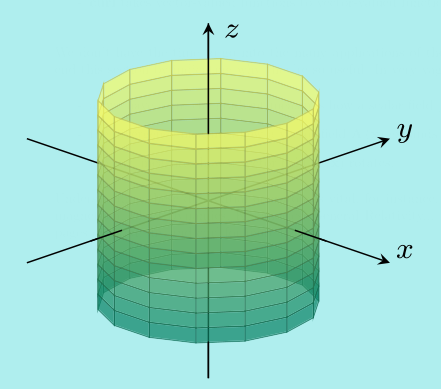
Here, there is no $z$ in the equation and $z$ takes arbitrary values. The horizontal cross sections are all circles $x^2+y^2=r^2$ with fixed radius $r$.

The paraboloid obtained by rotating a parabola about the $z$-axis: \[f(x,y,z)=x^2+y^2-z=0\]

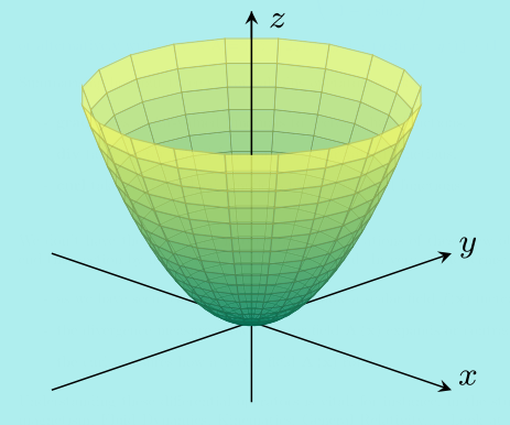
This time the horizontal cross sections are circles $x^2+y^2=z$ with radius $\sqrt{z}$ for any fixed $z$.

A (smooth) surface has a tangent plane and normal line at each point on the surface. We will next see how to write down the equations of this plane and line.

Let $S$ be a surface with equation $f(x,y,z)=C$ and ${\bf p}$ be a point on $S$. Furthermore, consider a curve which lies on $S$ and also passes through ${\bf p}$.

It can be written as ${\bf r}(t)=\left(x(t),y(t),z(t)\right)$ for some functions $x(t)$, $y(t)$ and $z(t)$ satisfying \[f\left({\bf r}(t)\right)=C.\] Differentiating this with respect to $t$ using the chain rule gives \[\begin{align*} \frac{df}{dt}=0 &\quad\implies\quad \frac{\partial f}{\partial x}\frac{dx}{dt}+\frac{\partial f}{\partial y}\frac{dy}{dt}+ \frac{\partial f}{\partial z}\frac{dz}{dt}=0 \\ &\quad\implies\quad \nabla f\cdot\frac{d{\bf r}}{dt}=0. \end{align*}\] So $\nabla f\left({\bf p}\right)$ is perpendicular to the curve at ${\bf p}$. But the surface $S$ around ${\bf p}$ is made up of all possible curves on $S$ through ${\bf p}$, and it follows that $\nabla f\left({\bf p}\right)$ is a normal vector to $S$ at ${\bf p}$. In particular, the normal line to $S$ through ${\bf p}$ has (parametric) equation \[{\bf x}={\bf p}+t\nabla f\left({\bf p}\right)\] and the tangent plane to $S$ at ${\bf p}$ has equation \[\left({\bf x}-{\bf p}\right)\cdot\nabla f\left({\bf p}\right)=0.\]

Example. $\,$ A sheet of metal is shaped to make a surface with equation \[f(x,y,z)=x^2+y^2+yz=0.\] A length of metal rod is welded to the sheet at two points with one end at $(2,-1,5)$ meeting the sheet at right angles. Find the other point of the sheet at which the metal rod should be attached. Also, find a Cartesian equation for the tangent plane to the surface at $(2,-1,5)$.

First check that $(2,-1,5)$ is on the surface: $f(2,-1,5)=4+1-5=0$.

Now \[\nabla f=\left(\dfrac{\partial f}{\partial x}, \dfrac{\partial f}{\partial y}, \dfrac{\partial f}{\partial z}\right)=2x{\bf i}+(2y+z){\bf j}+y{\bf k}\] and so \[\nabla f\left(2,-1,5\right)=4{\bf i}+3{\bf j}-{\bf k}.\] This means the normal has direction $4{\bf i}+3{\bf j}-{\bf k}$ and so the normal line through $(2,-1,5)$ has equation \[\frac{x-2}{4}=\frac{y+1}{3}=\frac{z-5}{-1}\] or, in parametric form, \[(x,y,z)=(2,-1,5)+t\left(4,3,-1\right)=(2+4t,-1+3t,5-t).\]

We need to find the values of $t$ for which these points lie on $S$, i.e. $x^2+y^2+yz=0$: \[\left(2+4t\right)^2+\left(-1+3t\right)^2+ \left(-1+3t\right)\left(5-t\right)=0 \] that is, $22t^2+26t=0$. This has two solutions: $t=0$ which corresponds to the point $(2,-1,5)$ and $t=-\dfrac{13}{11}$ which corresponds to the other intersection point, namely \[\left(2-\frac{52}{11},-1-\frac{39}{11},5+\frac{13}{11}\right)= \left(-\frac{30}{11},-\frac{50}{11},\frac{68}{11}\right). \]

Furthermore, the tangent plane through ${\bf p}=(2,-1,5)$ has equation $\left({\bf x}-{\bf p}\right)\cdot\nabla f\left({\bf p}\right)=0$. Using $\nabla f\left({\bf p}\right)=4{\bf i}+3{\bf j}-{\bf k}$, this rearranges to give the Cartesian equation \[4x+3y-z=4\times2+3(-1)-5=0.\]

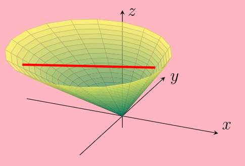
Actually, the surface $x^2+y^2+yz=0$ is a slanted cone. To see this, notice we can complete the square and rewrite as \[x^2+\left(y+\frac12z\right)^2=\frac14z^2.\] For each fixed $z$, the horizontal cross section at height $z$ is a circle of radius $\frac12z$ with centre at $(0,-z/2,z)$. Furthermore, we can see that the $z$-axis lies on the surface of the cone since $f(0,0,z)=0$ for all $z$.

5.6 Grad, Div and Curl: Vector fields

Recall that for a general function $f(x,y,z)$, we have the gradient \[ \nabla f=\left(\frac{\partial f}{\partial x}, \frac{\partial f}{\partial y}, \frac{\partial f}{\partial z}\right) ={\bf i}\frac{\partial f}{\partial x} +{\bf j}\frac{\partial f}{\partial y}+{\bf k}\frac{\partial f}{\partial z}. \] We can think of \[\nabla =\left(\frac{\partial }{\partial x}, \frac{\partial }{\partial y}, \frac{\partial }{\partial z}\right)={\bf i}\frac{\partial }{\partial x} +{\bf j}\frac{\partial }{\partial y}+{\bf k}\frac{\partial }{\partial z} \] as a vector in its own right - it’s a kind of hybrid of vector and differentiation which operates on the scalar-valued function $f$ to give the vector-valued function $\nabla f$. We will now see two other important ways of combining $\nabla$ with functions.

A function such as $f(x,y,z)$ above is often called a scalar field – it is a scalar-valued function $f\left({\bf x}\right)$ of a vector ${\bf x}=(x,y,z)$. We can also consider vector-valued functions of vectors: \[{\bf A}\left({\bf x}\right) = \left(A_1(x,y,z),A_2(x,y,z),A_3(x,y,z)\right).\] Such functions are called vector fields and are extremely important in many areas of Engineering and Science. For instance, consider a gravitational field. At every point ${\bf x}=(x,y,z)$ in space, there is a gravitational force and this is a vector with each component being a function of $x$, $y$ and $z$.

Now, we can combine two vectors ${\bf a}=\left( a_1,a_2,a_3\right)$ and ${\bf b}=\left( b_1,b_2,b_3\right)$ using the scalar product: \[{\bf a}\cdot{\bf b} = a_1b_1+a_2b_2+a_3b_3.\] This leads us to make the following definition.

Definition$\;$ The divergence of a vector field ${\bf A}\left({\bf x}\right) = \left(A_1(x,y,z),A_2(x,y,z),A_3(x,y,z)\right)$ is the scalar field \[\nabla\cdot {\bf A} =\left(\frac{\partial }{\partial x}, \frac{\partial }{\partial y}, \frac{\partial }{\partial z}\right) \cdot\left(A_1,A_2,A_3\right)=\frac{\partial A_1}{\partial x}+ \frac{\partial A_2}{\partial y}+ \frac{\partial A_3}{\partial z}. \]

(Note $\nabla\cdot {\bf A}$ is sometimes written ${\bf \operatorname{div}}\;A$. It is important to remember it is a scalar-valued function of vectors – look at the plus signs in the definition. If you miss them out then you’ve got it wrong!)

Examples. $\;$

$(1)\;$ Let ${\bf A}\left({\bf x}\right) =\left( x^2+yz,xyz^2,y^2-z^2\right)$. Then the divergence of ${\bf A}$ is \[\begin{align*} \nabla\cdot{\bf A} &=\left(\frac{\partial }{\partial x}, \frac{\partial }{\partial y}, \frac{\partial }{\partial z}\right) \cdot\left( x^2+yz,xyz^2,y^2-z^2\right) \\[1ex] &=\frac{\partial }{\partial x}\left( x^2+yz\right) + \frac{\partial }{ \partial y}\left(xyz^2\right) + \frac{\partial }{ \partial z}\left( y^2-z^2\right) \\[1ex] &= 2x+xz^2-2z. \end{align*}\]

$(2)\;$ Let ${\bf A}\left({\bf x}\right) =\left(yz\sin x,x+z^2\cos^2 y,xyz-\tan z\right)$. Then the divergence of ${\bf A}$ is \[\begin{align*} \nabla\cdot{\bf A} &=\left(\frac{\partial }{\partial x}, \frac{\partial }{\partial y}, \frac{\partial }{\partial z}\right) \cdot\left( yz\sin x,x+z^2\cos^2 y,xyz-\tan z\right)\\[1ex] &=\frac{\partial }{\partial x}\left(yz\sin x\right) + \frac{\partial }{ \partial y}\left(x+z^2\cos^2 y\right) + \frac{\partial }{ \partial z}\left(xyz-\tan z\right) \\[1ex] &= yz\cos x-2z^2\cos y\sin y+xy-\sec^2 z. \end{align*}\]

Another way to combine 3-dimensional vectors ${\bf a}=\left( a_1,a_2,a_3\right)$ and ${\bf b}=\left( b_1,b_2,b_3\right)$ is via the vector product: \[{\bf a}\times{\bf b} =\left|\begin{matrix} \textbf{i}&\textbf{j}&\textbf{k}\\ a_1&a_2&a_3\\ b_1&b_2&b_3 \end{matrix}\right| =\left( a_2b_3-a_3b_2\right)\textbf{i}+ \left( a_3b_1-a_1b_3\right)\textbf{j} +\left( a_1b_2-a_2b_1\right)\textbf{k}.\]

Using this, we are led to another definition:

Definition$\;$ The curl of a vector field ${\bf A}\left({\bf x}\right) = \left(A_1(x,y,z),A_2(x,y,z),A_3(x,y,z)\right)$ is the (vector-valued) function \[\begin{align*} \nabla\times{\bf A} &=\begin{pmatrix} {\partial}/{\partial x} \\ {\partial}/{\partial y} \\ {\partial}/{\partial z} \end{pmatrix} \times \begin{pmatrix} A_1 \\ A_2 \\ A_3 \end{pmatrix} = \left|\begin{matrix} \textbf{i}&\textbf{j}&\textbf{k}\\ \dfrac{\partial}{\partial x}&\dfrac{\partial}{\partial y}&\dfrac{\partial}{\partial z}\\ A_1&A_2&A_3 \end{matrix}\right| \\[1ex] &=\left(\frac{\partial A_3}{\partial y}-\frac{\partial A_2}{\partial z}\right)\textbf{i} +\left(\frac{\partial A_1}{\partial z}-\frac{\partial A_3}{\partial x}\right)\textbf{j} +\left(\frac{\partial A_2}{\partial x}-\frac{\partial A_1}{\partial y}\right)\textbf{k}. \end{align*}\]

(Note $\nabla\times {\bf A}$ is sometimes written ${\bf\operatorname{curl}}\;A$. It is important to remember it is a vector-valued function of vectors.)

Example. $\,$ It’s convenient to use column vectors for these calculations.

$(1)\;$ Let ${\bf A}\left({\bf x}\right) =\left( x^2+yz,xyz^2,y^2-z^2\right)$. Then the curl of ${\bf A}$ is \[\begin{align*} \nabla\times{\bf A}= \begin{pmatrix} {\partial}/{\partial x} \\ {\partial}/{\partial y} \\ {\partial}/{\partial z} \end{pmatrix} \times \begin{pmatrix} x^2+yz \\ xyz^2 \\ y^2-z^2 \end{pmatrix} &= \begin{pmatrix} \dfrac{\partial}{\partial y}\left(y^2-z^2\right)- \dfrac{\partial}{\partial z}\left(xyz^2\right)\\ \dfrac{\partial}{\partial z}\left( x^2+yz\right)- \dfrac{\partial}{\partial x}\left(y^2-z^2\right)\\ \dfrac{\partial}{\partial x}\left(xyz^2\right)- \dfrac{\partial}{\partial y}\left( x^2+yz\right) \end{pmatrix} \\ &=\begin{pmatrix} 2y-2xyz \\ y \\ yz^2-z \end{pmatrix} \end{align*}\] or alternatively written $\nabla\times{\bf A}= \left(2y-2xyz\right) \textbf{i}+y\textbf{j}+\left(yz^2-z\right)\textbf{k}$.

$(2)\;$ Let ${\bf A}\left({\bf x}\right) =\left(yz\sin x,x+z^2\cos^2 y,xyz-\tan z\right)$. Then the curl of ${\bf A}$ is \[\begin{align*} \nabla\times{\bf A}= \begin{pmatrix} {\partial}/{\partial x} \\ {\partial}/{\partial y} \\ {\partial}/{\partial z} \end{pmatrix} \times \begin{pmatrix} yz\sin x \\ x+z^2\cos^2 y \\ xyz-\tan z \end{pmatrix} &= \begin{pmatrix} \dfrac{\partial}{\partial y}\left(xyz-\tan z\right)- \dfrac{\partial}{\partial z}\left(x+z^2\cos^2 y\right)\\[3pt] \dfrac{\partial}{\partial z}\left(yz\sin x\right)- \dfrac{\partial}{\partial x}\left(xyz-\tan z\right)\\[3pt] \dfrac{\partial}{\partial x}\left(x+z^2\cos^2 y\right)- \dfrac{\partial}{\partial y}\left(yz\sin x\right) \end{pmatrix} \\ &=\begin{pmatrix} xz-2z\cos^2y \\ y\sin x-yz \\ 1-z\sin x \end{pmatrix} \end{align*}\] or alternatively written $\nabla\times{\bf A}=\left(xz-2z\cos^2y\right) \textbf{i}+\left(y\sin x-yz\right)\textbf{j} +\left(1-z\sin x\right)\textbf{k}$.

Summarising how our three vector calculus operators work:

${\bf grad}$ takes scalar-valued functions to vector-valued functions,
${\bf div}$ takes vector-valued functions to scalar-valued functions,
${\bf curl}$ takes vector-valued functions to vector-valued functions.

We don’t have the time to go into the many applications of these new objects but will end this section by indicating why they’re so useful. In very vague terms:

as we have seen, the gradient measures how a scalar field $f({\bf x})$ increases,
the divergence measures how a vector field ${\bf A}\left({\bf x}\right)$ expands or contracts,
the curl measures how a vector field ${\bf A}\left({\bf x}\right)$ rotates.

Understanding these differential operators is vital, for instance, in the study of Electromagnetism, Fluid Dynamics, Kinematics, General Relativity,… Look at the Wikipedia pages on grad, div and curl for more details if you are interested.

5.7 Critical points and Extreme values

Recall that for a function $f(x)$ of one variable, the points at which $df/dx=0$ are called critical points or stationary points. The tangent to the graph $y=f(x)$ at these points is horizontal. We also have the 2nd derivative test to decide if a critical point is a local maximum or minimum:

If $\dfrac{df}{ dx}=0$ and $\dfrac{d^2f}{ dx^2}>0$, then it’s a local minimum.
If $\dfrac{df}{dx}=0$ and $\dfrac{d^2f}{ dx^2}<0$, then it’s a local maximum.
If $\dfrac{df}{ dx}=0$ and $\dfrac{d^2f}{ dx^2}=0$, then the test is inconclusive.

We’ll now extend this to a function $f(x,y)$ of two variables. The graph of such a function is the surface $z=f(x,y)$ sitting above the $xy$ plane. Analogously to the case of functions of one variable, points at which \[\partial f/\partial x=\partial f/\partial y=0\] are called critical points and the tangent plane to the graph at these points is horizontal. This time, there are three types of critical points illustrated in the following simple examples.

Examples. $\;$

$(1)\;$ The surface $z=x^2+y^2$ is a paraboloid and the function \[f(x,y)=x^2+y^2\] has a local minimum when $(x,y)=(0,0)$. The value of $f$ at this point is $f(0,0)=0$.

$(2)\;$ The surface $z=1-x^2-y^2$ is also a paraboloid and the function \[f(x,y)=1-x^2-y^2\] has a local maximum when $(x,y)=(0,0)$. The value of $f$ at this point is $f(0,0)=1$.

$(3)\;$ The surface $z=y^2-x^2$ is a hyperbolic paraboloid and the function \[f(x,y)=y^2-x^2\] has a saddle point at $(x,y)=(0,0)$. The value of $f$ at this point is $f(0,0)=0$.

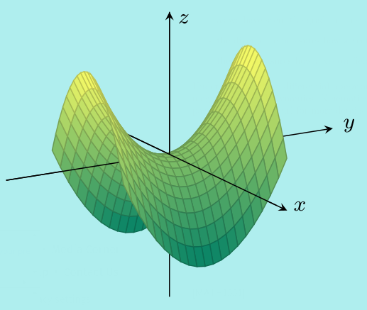
Notice a vertical cross section parallel to the $y$-axis is a parabola with a minimum, whereas a vertical cross section parallel to the $x$-axis is a a parabola with a maximum.

The 2nd partial derivative test can be used to determine if a critical point is a local minimum, local maximum or a saddle point. First define \[D(x,y)=\left(\dfrac{\partial^2 f}{\partial x^2}\right) \left(\dfrac{\partial^2 f}{\partial y^2}\right)- \left(\dfrac{\partial^2 f}{\partial y\partial x}\right)^2\] and suppose $(x,y)$ is a critical point, i.e. $\dfrac{\partial f}{\partial x}=\dfrac{\partial f}{\partial y}=0$.

If $D(x,y)>0$ and $\dfrac{\partial^2 f}{\partial x^2}>0$ then $(x,y)$ is a local minimum.
If $D(x,y)>0$ and $\dfrac{\partial^2 f}{\partial x^2}<0$ then $(x,y)$ is a local maximum.
If $D(x,y)<0$ then $(x,y)$ is a saddle point.
If $D(x,y)=0$, then the test is inconclusive.

Notice that \[\begin{align*} D(x,y)>0\quad\implies\quad \frac{\partial^2 f}{\partial x^2}\frac{\partial^2 f}{\partial y^2}&> \left(\frac{\partial^2 f}{\partial y\partial x}\right)^2\geq 0. \end{align*}\] Thus in the local maximum/minimum cases, $\dfrac{\partial^2 f}{\partial y^2}$ and $\dfrac{\partial^2 f}{\partial x^2}$ are either both positive or both negative and we can use either in the test.

The proof of this test uses a version of Taylor’s Theorem for functions of two variables. See any book on multi-variable calculus if you want to read a proof. The function $D(x,y)$ is the determinant of the Hessian matrix formed from the various 2nd derivatives \[\begin{pmatrix} \dfrac{\partial^2 f}{\partial x^2} & \dfrac{\partial^2 f}{\partial x\partial y} \\[3pt] \dfrac{\partial^2 f}{\partial y\partial x} & \dfrac{\partial^2 f}{\partial y^2} \end{pmatrix}.\]

Example. $\,$ Find all the critical points of the function \[f(x,y)=2x^3-x^2y+\frac{1}{2}y^2\] and where possible, classify each as a local maximum, local minimum, or saddle point.

We first calculate \[\frac{\partial f}{ \partial x}=6x^2-2xy\qquad\text{and}\qquad \frac{\partial f}{ \partial y}=-x^2+y\] and use these to locate the critical points: \[\begin{align*} 6x^2-2xy=0 \qquad & \text{and} \qquad -x^2+y=0 \\ \iff 2x(3x-y)=0 \qquad & \text{and} \qquad y=x^2 \\ \iff \text{$x=0$ or $3x=y=x^2$} \qquad & \text{and} \qquad y=x^2 \\ \iff \text{$x=0$ and $y=0$} \qquad & \text{or} \qquad y=x^2=3x \\ \iff (x,y)=(0,0) \qquad & \text{or} \qquad (x,y)=(3,9) \end{align*}\] Also, we have 2nd derivatives \[\frac{\partial^2 f}{\partial x^2}=12x-2y, \qquad \frac{\partial^2 f}{\partial y^2}=1\qquad\text{and}\qquad \frac{\partial^2 f}{\partial y\partial x}=-2x\] and so \[D(x,y)=(12x-2y)(1)-(-2x)^2=12x-2y-4x^2.\]

Now

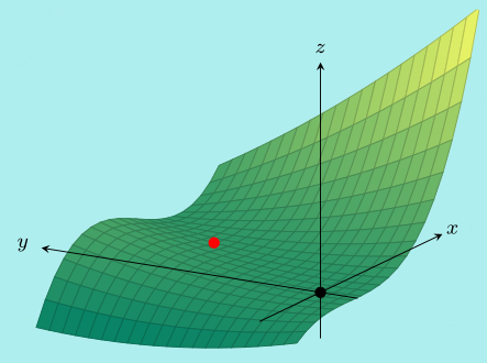
For the critical point $(0,0)$, we have $D(0,0)=0$ so the test is inconclusive here.
For the critical point $(3,9)$, we have $D(3,9)=36-18-4\times3^2=-18<0$ so $(3,9)$ is a saddle point.

Here’s a plot of the surface $z=f(x,y)$ with the saddle point in red.

Notation: When working with partial derivatives, the following notation is often useful: \[f_x =\frac{\partial f}{\partial x},\qquad f_{xx}=\frac{\partial^2 f}{\partial x^2},\qquad f_y =\frac{\partial f}{\partial y},\qquad f_{yy}=\frac{\partial^2 f}{\partial y^2}, \] \[f_{xy}=\frac{\partial}{\partial y}\left(\frac{\partial f}{\partial x}\right)= \frac{\partial^2 f}{\partial y\partial x}, \qquad f_{yx}=\frac{\partial^2 f}{\partial x\partial y}, \qquad\text{etc.}\]

Example. $\,$ Find all the critical points of the function $f(x,y)=y^2+\cos x$ and classify each as a local maximum, local minimum, or saddle point.

We calculate the first derivatives: \[ f_x=-\sin x\qquad\text{and}\qquad f_y=2y.\]

These are both zero when $x=n\pi$, $y=0$ for integer $n$ so the critical points are $(n\pi,0)$.

Also, the second derivatives are $f_{xx}=-\cos x$, $f_{yy}=2$, $f_{xy}=0$ and so \[D(x,y)=f_{xx}f_{yy}-f_{xy}^2=-2\cos{x}.\] Notice that $\cos(n\pi)=(-1)^n$ for integer $n$ so at the critical point $(n\pi,0)$, \[D(x,y)=2(-1)^{n+1} \quad\text{and}\quad f_{xx}=(-1)^{n+1}.\] We can now apply the test:

At $(n\pi,0)$ when $n$ is odd, we have $D(x,y)=2>0$ and $f_{xx}=1>0$, so this is a local minimum.
At $(n\pi,0)$ where $n$ is even, we have $D(x,y)=-2<0$, so this is a saddle point.

Here’s a plot of $z=y^2+\cos{x}$. Vertical cross-sections parallel to the $y$-axis are parabolas and vertical cross-sections parallel to the $x$-axis are cosine waves.

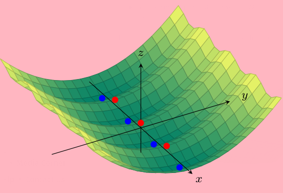
If you placed a ball at a local minimum (coloured blue) and gave it a little push, it would return to its position. If you balanced a ball at a saddle point (coloured red) and pushed it slightly in the $x$-direction, it would roll down the hill.