Topic 3 - Vectors

3.0 Introduction

Vectors are objects with both length and direction. We can think of a vector as an arrow from one place to another.

We will mostly consider them in 2- or 3-dimensional Euclidean space $\mathbb{R}^2$ or $\mathbb{R}^3$, but the concept is much more general.

Given two points $A$ and $B$ (in $\mathbb{R}^2$ or $\mathbb{R}^3$ or $\ldots$), the vector $\overrightarrow{AB}$ is the straight line path from $A$ to $B$. Vectors consist of both a direction and a length. We write $\left|\overrightarrow{AB}\right|$ for this length and, if this equals 1 we call it a unit vector.

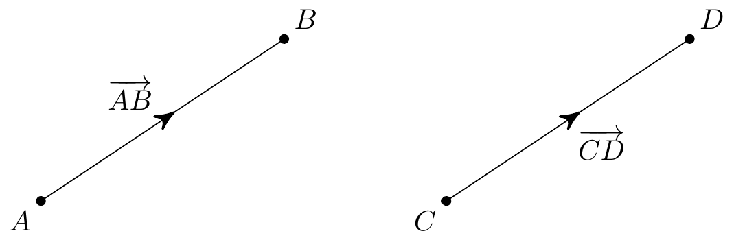
The vector doesn’t actually depend on the starting point and you should think of it as what you have to do to get from $A$ to $B$. So given a parallel path from $C$ to $D$ of the same length, we actually have $\overrightarrow{AB}=\overrightarrow{CD}$.

With the origin at $O$, the vector $\overrightarrow{OA}$ is called the position vector of $A$.

For convenience, if we don’t want to refer to two points, we just label vectors by a single letter. In these notes, we’ll use boldface letters like ${\bf u}$, ${\bf v}$. When writing by hand we often use underlined letters like $\underline{u}$, $\underline{v}$, or sometimes arrows like $\vec{u}$, $\vec{v}$.

Many fundamental quantities in science and engineering are most naturally described by vectors. These include positions, velocities and forces in particle mechanics (which we will mention briefly later). In future courses you may learn about vector fields, where there is a vector defined at every point in space. These include quantities such as the velocity field in fluid mechanics, the electric and magnetic fields in electromagnetism, or the Earth’s gravitational field.

3.1 Basic Rules

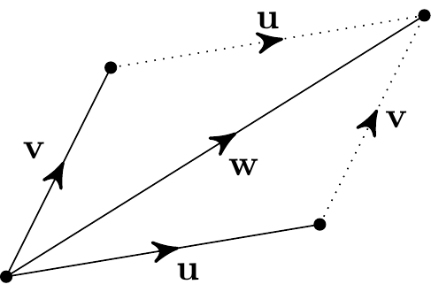
Vector addition. $\;$ We add vectors “head to tail”. Thus we always have

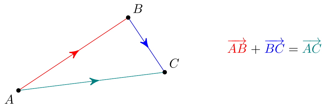
With two vectors ${\bf u}$ and ${\bf v}$, the sum ${\bf w} = {\bf u} + {\bf v}$ is the path to the corner of the parallelogram formed from ${\bf u}$ and ${\bf v}$:

Scalar multiplication. $\;$ We can multiply a vector ${\bf u}$ by a $\lambda\in\mathbb{R}$ to give a new vector $\lambda{\bf u}$. This is in the same direction as ${\bf u}$ for $\lambda > 0$ and in the opposite direction if $\lambda <0$, and the length is scaled by $|\lambda|$, so \[ |\lambda{\bf u}| = |\lambda|\,|{\bf u}|. \]

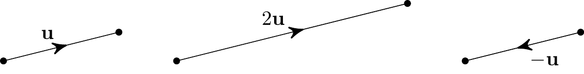
If ${\bf u}$ is parallel to ${\bf v}$, then ${\bf v}=\lambda{\bf u}$ for some $\lambda\neq 0$.
If $\lambda{\bf u}=\mu{\bf v}$ and ${\bf u}$ is not parallel to ${\bf v}$, then it must be that $\lambda=\mu=0$.

Vector addition and scalar multiplication satisfy the following rules (similar to addition and multiplication of real numbers):

Commutativity: ${\bf u} + {\bf v} = {\bf v} + {\bf u}$.
Associativity: ${\bf u} + ({\bf v} + {\bf w}) = ({\bf u} + {\bf v}) + {\bf w}$.
Distributivity: $(\lambda + \mu){\bf u} = \lambda{\bf u} + \mu{\bf u}$, $\quad\lambda({\bf u} + {\bf v}) = \lambda{\bf u} + \lambda{\bf v}$, $\quad\lambda(\mu{\bf u}) = (\lambda\mu){\bf u}$.

We also have a zero vector $\boldsymbol{0}$. (This doesn’t have a direction but we call it a “vector” anyway!) It satisfies ${\bf u} + \boldsymbol{0}={\bf u}$ for every ${\bf u}$ and has length $0$.

Example. $\,$ If the position vectors of $A$, $B$ and $C$ are ${\bf a}$, ${\bf b}$ and $2{\bf a} + 3{\bf b}$ respectively, what are $\overrightarrow{AB}$, $\overrightarrow{BC}$ and $\overrightarrow{CA}$? \[\begin{align*} \overrightarrow{AB}&=\overrightarrow{AO}+\overrightarrow{OB}= \overrightarrow{OB}-\overrightarrow{OA}={\bf b}-{\bf a} \\ \overrightarrow{BC}&=\overrightarrow{OC}-\overrightarrow{OB}= 2{\bf a}+3{\bf b}-{\bf b}=2{\bf a}+2{\bf b} \\ \overrightarrow{CA}&=\overrightarrow{OA}-\overrightarrow{OC}= {\bf a}-(2{\bf a}+3{\bf b})=-{\bf a}-3{\bf b} \end{align*}\]

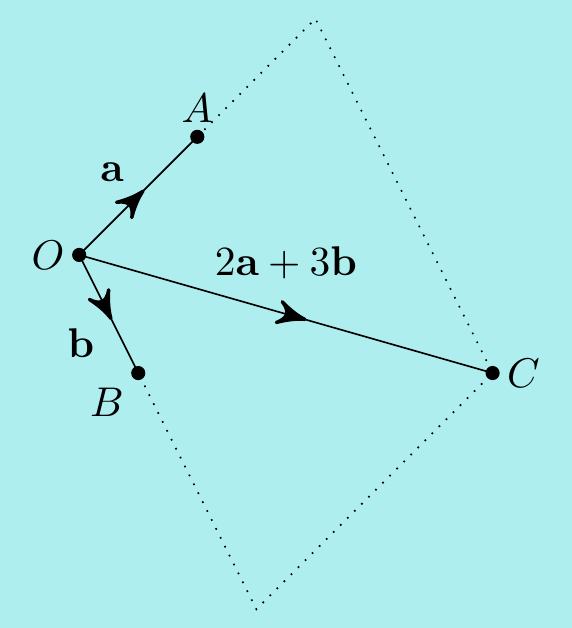
Notice that $\overrightarrow{AB}+\overrightarrow{BC}+\overrightarrow{CA}=\boldsymbol{0}$. Going from $A$ to $B$ to $C$ to $A$ goes nowhere!

Let’s look at a more interesting example.

Example. $\,$ Given a triangle $ABC$, show that the three lines connecting $A$ to the midpoint of $BC$, $B$ to the midpoint of $CA$ and $C$ to the midpoint of $AB$ intersect at a common point. Furthermore, show that the intersection is $2/3$ of the way along each of these lines.

Let the three midpoints be $D$, $E$ and $F$ as shown below, and let $X$ be the point where $BE$ and $CF$ intersect. We want to show that $X$ lies on $AD$.

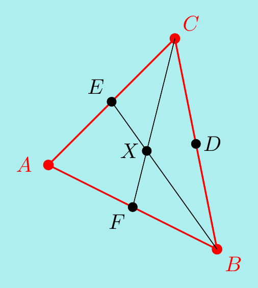
Let ${\bf u}=\overrightarrow{AB}$ and ${\bf v}=\overrightarrow{AC}$. Then $\overrightarrow{BC}={\bf v}-{\bf u}$ and the three lines have vectors \[\begin{align*} \overrightarrow{AD}&=\overrightarrow{AB}+\frac12\overrightarrow{BC} ={\bf u}+\frac12({\bf v}-{\bf u})=\frac12{\bf v}+\frac12{\bf u}, \\ \overrightarrow{BE}&=\overrightarrow{BA}+\frac12\overrightarrow{AC} =-{\bf u}+\frac12{\bf v}, \\ \overrightarrow{CF}&=\overrightarrow{CA}+\frac12\overrightarrow{AB} =-{\bf v}+\frac12{\bf u}. \end{align*}\] We will now express $\overrightarrow{AX}$ in two ways. Notice $\overrightarrow{BX}=\lambda\overrightarrow{BE}$ and $\overrightarrow{CX}=\mu\overrightarrow{CF}$ for some $\mu,\lambda$. Thus \[\begin{align*} \overrightarrow{AX} =\overrightarrow{AB}+\overrightarrow{BX} &=\overrightarrow{AB}+\lambda\overrightarrow{BE}\\ &={\bf u}+\lambda\left(-{\bf u}+\frac12{\bf v}\right) =(1-\lambda){\bf u}+\frac12\lambda{\bf v}. \end{align*}\] Similarly, \[\begin{align*} \overrightarrow{AX} =\overrightarrow{AC}+\overrightarrow{CX} &=\overrightarrow{AC}+\mu\overrightarrow{CF}\\ &={\bf v}+\mu\left(-{\bf v}+\frac12{\bf u}\right) =(1-\mu){\bf v}+\frac12\mu{\bf u}. \end{align*}\] Equating these gives \[\begin{align*} (1-\lambda){\bf u}+\frac12\lambda{\bf v} &=(1-\mu){\bf v}+\frac12\mu{\bf u}\\ \implies\quad \left(1-\lambda-\frac12\mu\right){\bf u} &=\left(1-\mu-\frac12\lambda\right){\bf v}. \end{align*}\] However, ${\bf u}$ and ${\bf v}$ are not parallel (if they were, the triangle would collapse into a line and the question would be much easier). So the above equation must say $0{\bf u}=0{\bf v}$ and \[ \left\{\begin{matrix} 1-\lambda-\frac12\mu = 0 \\[5pt] 1-\mu-\frac12\lambda = 0 \end{matrix}\right. \quad\implies \lambda=\mu=\frac23. \] In particular, $\overrightarrow{BX}=\dfrac23\overrightarrow{BE}$ and $\overrightarrow{CX}=\dfrac23\overrightarrow{CF}$.

Furthermore, using the above formulas for $\overrightarrow{AX}$ and $\overrightarrow{AD}$, we have \[\overrightarrow{AX}=\dfrac13{\bf u}+\dfrac13{\bf v}= \dfrac23\overrightarrow{AD}\] and $X$ lies $2/3$ of the way along on $AD$, $BE$ and $CF$.

The point $X$ is called the centroid of the triangle $ABC$. If we make the triangle out of a thin, uniform density sheet of metal, then $X$ is the centre of mass.

3.2 Coordinates and Bases

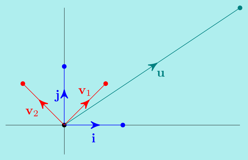
We often represent vectors by using coordinates. For example, consider the following vector in $\mathbb{R}^2$

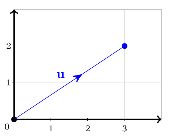
It can be represented as ${\bf u} = \displaystyle\begin{pmatrix} 3 \\ 2 \end{pmatrix}$, in the same form we used in the Linear Algebra topic.

An alternative notation uses the standard basis vectors ${\bf i} = \begin{pmatrix} 1 \\ 0 \end{pmatrix}$ and ${\bf j} = \begin{pmatrix} 0 \\ 1 \end{pmatrix}$. We can write ${\bf u} = 3{\bf i} + 2{\bf j}$ and we call $3$ and $2$ the of the vector with respect to the standard basis. By Pythagoras’ Theorem the length of this vector is $|{\bf u}| = \sqrt{2^2 + 3^2}=\sqrt{13}.$

Adding two vectors just corresponds to adding the coordinates: \[ \begin{pmatrix} 3 \\ 2 \end{pmatrix} + \begin{pmatrix} 1 \\ -1 \end{pmatrix} = \begin{pmatrix} 4 \\ 1 \end{pmatrix}\] or in terms of the standard basis vectors $\left(3{\bf i} + 2{\bf j}\right) + \left({\bf i}-{\bf j}\right)= 4{\bf i} + {\bf j}$.

Multiplying by a scalar just multiplies the coordinates: \[ 4\begin{pmatrix} 3 \\ 2\end{pmatrix} = \begin{pmatrix} 4\times 3\\ 4\times 2\end{pmatrix} = \begin{pmatrix} 12 \\ 8\end{pmatrix}\] or alternatively, we can write $4\left(3{\bf i} + 2{\bf j}\right) = 12{\bf i} + 8{\bf j}$.

Similarly, a vector in $\mathbb{R}^3$ can be written \[ {\bf u} = \begin{pmatrix} x\\y\\z \end{pmatrix} = x\begin{pmatrix} 1\\0\\0 \end{pmatrix} + y\begin{pmatrix} 0\\1\\0 \end{pmatrix} + z\begin{pmatrix} 0\\0\\1 \end{pmatrix} = x{\bf i} + y{\bf j} + z{\bf k}. \] It has length $|{\bf u}|=\sqrt{x^2 + y^2 + z^2}$ and addition/scalar multiplication work in the obvious way.

An $n$-dimensional vector in $n$-dimensional space $\mathbb{R}^n$ is handled in the same way: it has $n$ coordinates with respect to $n$ standard basis vectors (often called ${\bf e}_1,{\bf e}_2,\ldots,{\bf e}_n$, where ${\bf e}_i$ has a $1$ in the $i$-th coordinate and $0$ everywhere else).

Notice that vectors are nothing other than matrices with a single column. But now they have geometric meaning as well.

Sometimes, it’s useful to write a vector in terms of other vectors, rather than the standard basis. Given a set of $m$ vectors $S=\{{\bf v}_1,{\bf v}_2,...,{\bf v}_m\}$ in $n$-dimensional space $\mathbb{R}^n$, the span of the vectors, written as $\operatorname{Span}(S)$, is the set of all linear combinations \[ {\bf u} = c_1{\bf v}_1 + c_2{\bf v}_2 + \ldots +c_m{\bf v}_m \quad\text{for $c_1$, $c_2$, \ldots $c_m \in \mathbb{R}$}. \] We say that the set spans $\mathbb{R}^n$ if every vector in $\mathbb{R}^n$ can be written in this way. It means we can reach every point using the directions of the set $S$ in at least one way.

Example. $\,$

$(1)\;$ Consider the vectors ${\bf v}_1=\begin{pmatrix} 2 \\ 0 \\ 0 \end{pmatrix}$, ${\bf v}_2=\begin{pmatrix} 0 \\ 3 \\ 0 \end{pmatrix}$ in $\mathbb{R}^3$.

We can see directly that $c_1\begin{pmatrix} 2 \\ 0 \\ 0 \end{pmatrix} +c_2\begin{pmatrix} 0 \\ 3 \\ 0 \end{pmatrix} =\begin{pmatrix} 2c_1 \\ 3c_2 \\ 0 \end{pmatrix}$, which can’t equal e.g. $\begin{pmatrix} 0 \\ 0 \\ 1 \end{pmatrix}$.

Hence these vectors don’t span $\mathbb{R}^3$. More generally, there’s no way that less than 3 vectors could span $\mathbb{R}^3$. We can’t get everywhere in 3-d space using only two directions.

$(2)\;$ Consider the vectors ${\bf v}_1=\begin{pmatrix} 0 \\ 1 \\ 2 \end{pmatrix}$, ${\bf v}_2=\begin{pmatrix} 2 \\ 0 \\ 1 \end{pmatrix}$, ${\bf v}_3=\begin{pmatrix} 1 \\ 2 \\ 0 \end{pmatrix}$ in $\mathbb{R}^3$.

Spanning means we can find $c_1,c_2,c_3$ so that $c_1{\bf v}_1+c_2{\bf v}_2+c_3{\bf v}_3={\bf u}$ for arbitrary ${\bf u}$. Notice we can rewrite this as a matrix equation \[\begin{align*} c_1\begin{pmatrix} 0 \\ 1 \\ 2 \end{pmatrix} +c_2\begin{pmatrix} 2 \\ 0 \\ 1 \end{pmatrix} +c_3\begin{pmatrix} 1 \\ 2 \\ 0 \end{pmatrix} =\begin{pmatrix} 0 & 2 & 1 \\ 1 & 0 & 2 \\ 2 & 1 & 0 \end{pmatrix} \begin{pmatrix} c_1 \\ c_2 \\ c_3\end{pmatrix} =\begin{pmatrix} u \\ v \\ w \end{pmatrix}. \end{align*}\]

We can check the determinant of the matrix is non-zero, so it is invertible and there is a solution. In other words, this set does span $\mathbb{R}^3$.

$(3)\;$ Be careful though - a set with at least $3$ vectors does necessarily span $\mathbb{R}^3$.

For instance, $S=\left\{\begin{pmatrix} 1 \\ 1 \\ 1 \end{pmatrix}, \begin{pmatrix} 2 \\ 2 \\ 2 \end{pmatrix}, \begin{pmatrix} 3 \\ 3 \\ 3 \end{pmatrix}, \begin{pmatrix} 4 \\ 4 \\ 4 \end{pmatrix}\right\}$ clearly doesn’t.

Another very useful concept is linear independence. A set of $m$ vectors $S=\{{\bf v}_1,{\bf v}_2,...,{\bf v}_m\}$ is called linearly independent if none of the vectors is a linear combination of the others. An alternative way of saying this is that \[ c_1{\bf v}_1 + c_2{\bf v}_2 + \ldots + c_m{\bf v}_m \quad\iff\quad c_1=c_2\ldots=c_n=0. \] This essentially says there are no redundant directions in the set $S$ and we can reach a particular point in space in at most one way (though possibly not at all). \[\begin{align*} & c_1{\bf v}_1+c_2{\bf v}_2+...+c_m{\bf v}_m=d_1{\bf v}_1+d_2{\bf v}_2+...+d_m{\bf v}_m \qquad\qquad \\ &\qquad\qquad\iff\quad (c_1-d_1){\bf v}_1+(c_2-d_2){\bf v}_2+...+(c_m-d_m){\bf v}_m={\bf 0} \\ &\qquad\qquad\iff\quad c_1-d_1=c_2-d_2=...=c_m-d_m=0 \\ &\qquad\qquad\iff\quad c_1=d_1,\; c_2=d_2,\;...\;,c_m=d_m. \end{align*}\]

Example. $\,$

$(1)\;$ Consider the vectors ${\bf v}_1=\begin{pmatrix} 1 \\ 0 \\ 0 \end{pmatrix}$, ${\bf v}_2=\begin{pmatrix} 0 \\ 1 \\ 0 \end{pmatrix}$, ${\bf v}_3=\begin{pmatrix} 0 \\ 0 \\ 1 \end{pmatrix}$, ${\bf v}_4=\begin{pmatrix} 1 \\ 2 \\ 3 \end{pmatrix}$.

We can see directly that ${\bf v}_1+2{\bf v}_2+3{\bf v}_3-{\bf v}_4={\bf 0}$ so they are not linearly independent.

More generally, there’s no way that more than 3 vectors in $\mathbb{R}^3$ can be linearly independent. We’ll always be able to write one of them in terms of the others.

Linear independence means that if $c_1{\bf v}_1+c_2{\bf v}_2+c_3{\bf v}_3={\bf 0}$, then $c_1=c_2=c_3=0$.

Again, we can rewrite this as a matrix equation \[\begin{align*} c_1\begin{pmatrix} 0 \\ 1 \\ 2 \end{pmatrix} +c_2\begin{pmatrix} 2 \\ 0 \\ 1 \end{pmatrix} +c_3\begin{pmatrix} 1 \\ 2 \\ 0 \end{pmatrix} =\begin{pmatrix} 0 & 2 & 1 \\ 1 & 0 & 2 \\ 2 & 1 & 0 \end{pmatrix} \begin{pmatrix} c_1 \\ c_2 \\ c_3\end{pmatrix} =\begin{pmatrix} 0 \\ 0 \\ 0 \end{pmatrix}. \end{align*}\]

The determinant of the matrix is non-zero, so there is a solution. But we can see that $c_1=c_2=c_3=0$ is a solution so it must be the only one! In other words, this set is linearly independent.

$(3)\;$ Be careful though - a set with less than $3$ vectors in $\mathbb{R}^3$ is necessarily linearly independent.

For instance, $S=\left\{\begin{pmatrix} 1 \\ 1 \\ 1 \end{pmatrix}, \begin{pmatrix} 2 \\ 2 \\ 2 \end{pmatrix}\right\}$ clearly isn’t.

So a set of vectors spans $\mathbb{R}^n$ if you can use them to reach everywhere in at least one way and it is linearly independent if you can only use them to get somewhere in at most one way. A basis is a set which both spans the space and is linearly independent.

Example. $\,$ The vectors ${\bf v}_1=\begin{pmatrix} 0 \\ 1 \\ 2 \end{pmatrix}$, ${\bf v}_2=\begin{pmatrix} 2 \\ 0 \\ 1 \end{pmatrix}$, ${\bf v}_3=\begin{pmatrix} 1 \\ 2 \\ 0 \end{pmatrix}$ form a basis of $\mathbb{R}^3$.

We’ve seen in the previous examples that they span $\mathbb{R}^3$ and are linearly independent.

Now, for a set of $m$ vectors $S=\{{\bf v}_1,{\bf v}_2,...,{\bf v}_m\}$ in $n$-dimensional space, we have

if $m<n$ then it can not span $\mathbb{R}^n$,
if $m>n$, then it can not be linearly independent.

In particular, a basis must have $m=n$, i.e. the same number of vectors as the dimension. Furthermore, there is exactly one way to write any given vector ${\bf u}\in\mathbb{R}^n$ as \[{\bf u}=c_1{\bf v}_1+c_2{\bf v}_2+\ldots+c_n{\bf v}_n\] We call $c_1,c_2,\ldots,c_n$ the coordinates of ${\bf u}$ with respect to the basis $\{{\bf v}_1,{\bf v}_2,...,{\bf v}_n\}$.

There is a quick way to check if a set $S$ of exactly $n$ vectors in $\mathbb{R}^n$ is a basis. In this case, the following are equivalent:

$S$ is linearly independent,
$S$ spans $\mathbb{R}^n$,
$S$ is a basis of $\mathbb{R}^n$,
the matrix with the vectors of $S$ as columns has determinant, i.e. is invertible.

Example. $\,$ Show that the vectors ${\bf v}_1=\begin{pmatrix} \frac{1}{\sqrt{2}} \\ \frac{1}{\sqrt{2}} \end{pmatrix}$ and ${\bf v}_2=\begin{pmatrix} -\frac{1}{\sqrt{2}} \\ \frac{1}{\sqrt{2}} \end{pmatrix}$ form a basis for $\mathbb{R}^2$, and find the coordinates of ${\bf u}=\begin{pmatrix} 3 \\ 2 \end{pmatrix}$ with respect to this basis.

To show it is a basis, we just need to check the determinant \[\begin{vmatrix} \frac{1}{\sqrt{2}} & -\frac{1}{\sqrt{2}} \\ \frac{1}{\sqrt{2}} & \frac{1}{\sqrt{2}} \end{vmatrix}=\frac12+\frac12=1\neq 0. \] To find the coordinates of ${\bf u}$ with respect to this new basis, write $c_1{\bf v}_1 + c_2{\bf v}_2={\bf u}$, so \[ c_1\begin{pmatrix} \frac{1}{\sqrt{2}} \\ \frac{1}{\sqrt{2}} \end{pmatrix} + c_2\begin{pmatrix} -\frac{1}{\sqrt{2}} \\ \frac{1}{\sqrt{2}} \end{pmatrix} = \begin{pmatrix} \frac{1}{\sqrt{2}} & -\frac{1}{\sqrt{2}} \\ \frac{1}{\sqrt{2}} & \frac{1}{\sqrt{2}} \end{pmatrix} \begin{pmatrix} c_1 \\ c_2 \end{pmatrix} = \begin{pmatrix} 3 \\ 2 \end{pmatrix}, \] and solve for the coordinates $c_1$ and $c_2$ (by Gaussian elimination or directly). We have \[ \left\{\begin{matrix} c_1-c_2 = 3\sqrt{2} \\ c_1+c_2 = 2\sqrt{2} \end{matrix}\right. \quad\implies c_1=\frac{5\sqrt{2}}{2}, \quad c_2=-\frac{\sqrt{2}}{2}. \]

Changing to a different basis thus corresponds to using a different coordinate system. This can simplify calculations and is useful in many applications in engineering and science.

3.3 The Scalar Product

The scalar product is a way of multiplying two vectors to get a scalar.

Given two vectors in $\mathbb{R}^2$, \[ {\bf u} = \begin{pmatrix} u_1\\u_2 \end{pmatrix} = u_1{\bf i} + u_2{\bf j} \quad \textsf{and} \quad {\bf v} = \begin{pmatrix} v_1\\v_2 \end{pmatrix} = v_1{\bf i} + v_2{\bf j}, \] their scalar product (also called dot product or inner product) is defined by \[ {\bf u}\cdot{\bf v} = u_1v_1 + u_2v_2. \]

Similarly for two vectors in $\mathbb{R}^3$, ${\bf u} = u_1{\bf i} + u_2{\bf j} + u_3{\bf k}$ and ${\bf v} = v_1{\bf i} + v_2{\bf j} + v_3{\bf k}$, their scalar product is ${\bf u}\cdot{\bf v} = u_1v_1 + u_2v_2 + u_3v_3$.

You should be able to guess how to define it for $n$-dimensional vectors – just multiply the corresponding coordinates and add.

The scalar product has the following nice, natural properties:

Commutativity: ${\bf u}\cdot{\bf v} = {\bf v}\cdot{\bf u}$.
Scalar associativity: $(\lambda{\bf u})\cdot{\bf v} = \lambda({\bf u}\cdot{\bf v})$.
Distributivity: ${\bf u}\cdot({\bf v}+{\bf w}) = {\bf u}\cdot{\bf v} + {\bf u}\cdot{\bf w}$.
Length: ${\bf u}\cdot{\bf u} = |{\bf u}|^2$.
Perpendicularity: ${\bf u}\cdot{\bf v}=0$ if and only if ${\bf u}$ and ${\bf v}$ are perpendicular.

The first four properties follow readily from the definition. The last property is a special case of the important formula \[ {\bf u}\cdot{\bf v} = |{\bf u}|\,|{\bf v}|\cos\theta \] where $\theta$ is the angle between ${\bf u}$ and ${\bf v}$. We can prove it using the cosine law: this is a generalisation of Pythagoras’s Theorem to non-right-angled triangles.

Suppose a triangle has side lengths $a$, $b$, $c$ and angle $\theta$ as shown.

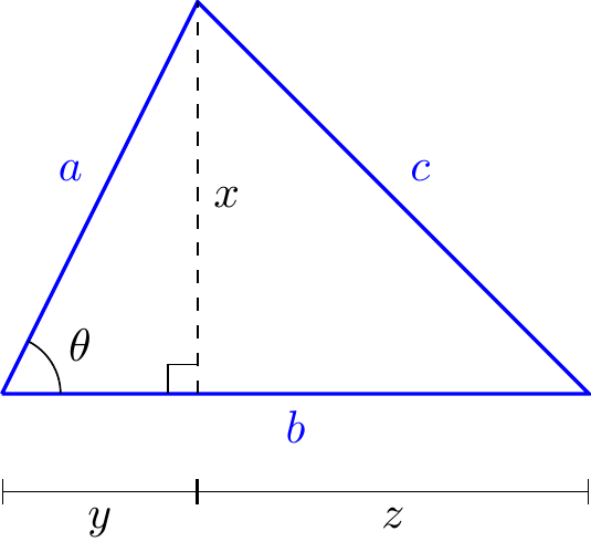
Split it into two smaller right-angled triangles as shown and use Pythagoras’s Theorem on each of these: \[\begin{align*} c^2=x^2+z^2=x^2+(b-y)^2&=x^2+y^2+b^2-2by \\ &=a^2+b^2-2by \\ &=a^2+b^2-2ab\cos\theta. \end{align*}\] Now consider the triangle formed by two vectors ${\bf u}$ and ${\bf v}$

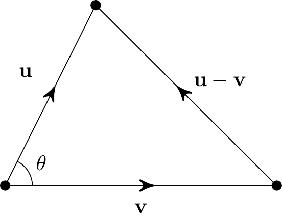
It has side lengths $a=|{\bf u}|$, $b=|{\bf v}|$ and $c=|{\bf u}-{\bf v}|$, so using the cosine law, we get \[|{\bf u}-{\bf v}|^2=|{\bf u}|^2+|{\bf v}|^2-2|{\bf u}|\,|{\bf v}|\cos\theta.\] Also, using the properties of the scalar product, \[\begin{align*} |{\bf u}-{\bf v}|^2 &= \left({\bf u}-{\bf v}\right)\cdot\left({\bf u}-{\bf v}\right) \\ &= {\bf u}\cdot{\bf u}+{\bf v}\cdot{\bf v}-{\bf u}\cdot{\bf v}-{\bf v}\cdot{\bf u} \\ &= |{\bf u}|^2+|{\bf v}|^2-2{\bf u}\cdot{\bf v}. \end{align*}\] Comparing these two formulas gives ${\bf u}\cdot{\bf v} = |{\bf u}|\,|{\bf v}|\cos\theta$.

This formula gives us an easy way to calculate angles between vectors.

Example. $\,$ Find the angle between the vectors \[{\bf u}=\begin{pmatrix} 1 \\ 1 \\ 1 \end{pmatrix} = {\bf i} + {\bf j} + {\bf k} \quad\text{and}\quad {\bf v}=\begin{pmatrix} 2 \\ 0 \\ -3 \end{pmatrix} = 2{\bf i} - 3{\bf k}. \] We have \[\begin{align*} {\bf u}\cdot{\bf v} &= 1(2) + 1(0) + 1(-3) = -1,\\ |{\bf u}| &= \sqrt{1^2 + 1^2 + 1^2} = \sqrt{3},\\ |{\bf v}| &= \sqrt{2^2 + 0^2 + (-3)^2} = \sqrt{13}, \end{align*}\] so \[ \cos\theta = \frac{{\bf u}\cdot{\bf v}}{|{\bf u}|\,|{\bf v}|} = \frac{-1}{\sqrt{3}\sqrt{13}} \quad \implies \theta=\arccos\left(\frac{-1}{\sqrt{39}}\right). \]

3.4 Projections and Orthonormality

Another way to think about the scalar product is in terms of projections. Given two vectors ${\bf a}=\overrightarrow{OA}$ and ${\bf b}=\overrightarrow{OB}$, there is a point $C$ on $OB$ with $AC$ perpendicular to $OB$.

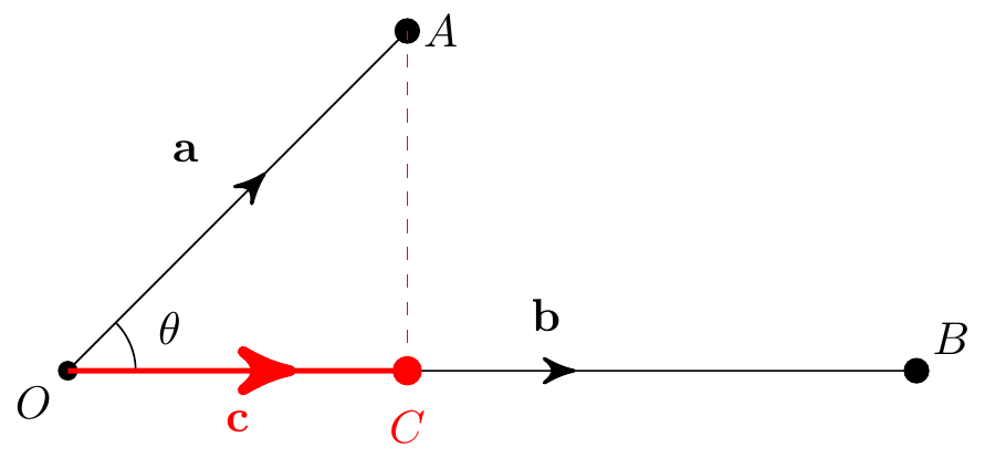
Then the projection of ${\bf a}$ onto ${\bf b}$ is the vector ${\bf c}=\overrightarrow{OC}$. Its length $|\overrightarrow{OC}|$ is the component of ${\bf a}$ in the direction of ${\bf b}$, and is given by \[ |\overrightarrow{OC}| = |{\bf a}|\cos\theta = |{\bf a}|\frac{{\bf a}\cdot{\bf b}}{|{\bf a}|\,|{\bf b}|} = \frac{{\bf a}\cdot{\bf b}}{|{\bf b}|}. \]

The projection ${\bf c}$ is a multiple of ${\bf b}$, but which multiple? A unit vector in the direction of ${\bf b}$ is ${\bf b}/|{\bf b}|$, so we can write the projection vector as \[ {\bf c} = \left(\frac{{\bf a}\cdot{\bf b}}{|{\bf b}|}\right) \frac{{\bf b}}{|{\bf b}|} = \left(\frac{{\bf a}\cdot{\bf b}}{|{\bf b}|^2}\right){\bf b}. \]

The projection is essentially telling us how much ${\bf a}$ goes in the direction of ${\bf b}$.

There is a related application of the scalar product in physics/engineering. The work done (energy used up) by a force ${\bf F}$ moving a particle through a displacement ${\bf d}$ is \[ W = {\bf F}\cdot{\bf d}. \] It’s the component of the force in the direction of motion, multiplied by the distance $|{\bf d}|$.

Example. $\,$ A particle is displaced ${\bf d}=2{\bf i} + 3{\bf j}$ by a force ${\bf F}={\bf i}+{\bf j}$. The work done on the particle by the force is just \[ W = {\bf F}\cdot{\bf d} = (2{\bf i} + 3{\bf j})\cdot({\bf i} + {\bf j}) = 2(1) + 3(1) = 5. \]

A nice property of the standard basis vectors such as ${\bf i}$, ${\bf j}$, ${\bf k}$ in $\mathbb{R}^3$ is that they are all unit length and mutually perpendicular. That is, \[ {\bf i}\cdot{\bf i} = {\bf j}\cdot{\bf j} = {\bf k}\cdot{\bf k} =1 \] and \[ {\bf i}\cdot{\bf j} = {\bf i}\cdot{\bf k} = {\bf j}\cdot{\bf k} = 0. \]

A basis of mutually perpendicular unit vectors is called orthonormal.

Example. $\,$ The basis ${\bf v}_1=(\cos\theta){\bf i} + (\sin\theta){\bf j}$, ${\bf v}_2= (-\sin\theta){\bf i} + (\cos\theta){\bf j}$ of $\mathbb{R}^2$.

We can check that this basis is orthonormal: \[\begin{align*} &{\bf v}_1\cdot{\bf v}_1 = \cos^2\theta + \sin^2\theta = 1,\\ &{\bf v}_2\cdot{\bf v}_2 = \sin^2\theta + \cos^2\theta = 1,\\ &{\bf v}_1\cdot{\bf v}_2 = -\cos\theta\sin\theta + \sin\theta\cos\theta = 0. \end{align*}\]

Notice that ${\bf v}_1$ and ${\bf v}_2$ are just the vectors obtained by rotating ${\bf i}$ and ${\bf j}$ anti-clockwise about the origin by angle $\theta$.

The concept of vectors goes far beyond the Euclidean spaces $\mathbb{R}^n$ we consider in this course. Ideas such as scalar products and orthonormal bases work in much more generality.

A particular example you may meet later in your course is Fourier series. Functions which are both odd and periodic with period $2\pi$, i.e. \[f(-x)=-f(x)\qquad\text{and}\qquad f(x+2\pi) = f(x)\] can be thought of as vectors in an infinite-dimensional vector space. We can add them, multiply by scalars,…, just as we do with ordinary vectors. A basis for this vector space of functions is \[\{\sin x, \sin(2x), \sin(3x),\ldots\},\] and every function of this type (almost) can be written as an infinite sum \[ f(x) = a_1\sin x + a_2\sin(2x) + a_3\sin(3x) + \ldots = \sum_{n=1}^\infty a_n\sin(nx) \] for some real numbers $a_1, a_2,\ldots$. The scalar product in this case is \[ f \cdot g = \frac{1}{\pi}\int_{-\pi}^\pi f(x)g(x)\,\mathrm{d}x \] and one can show that \[ \sin(mx)\cdot\sin(nx) = \frac{1}{\pi}\int_{-\pi}^\pi\sin(mx)\sin(nx)\,\mathrm{d}x = \left\{\begin{matrix}1 \quad \textrm{if $m=n$}\\ 0 \quad \textrm{if $m\neq n$} \end{matrix}\right. \] so that the basis $\{\sin x, \sin(2x), \sin(3x),\ldots\}$ is actually orthonormal.

These kind of functions are useful wherever oscillatory behaviour appears – for example, vibrating strings, signal processing or quantum mechanics.

3.5 Lines in 3 dimensions

We can write the equation for a straight line in terms of vectors. Given two points $A$ and $B$ with position vectors ${\bf a}$ and ${\bf b}$ respectively, the direction of the line joining $A$ and $B$ has direction ${\bf d}={\bf b}-{\bf a}$.

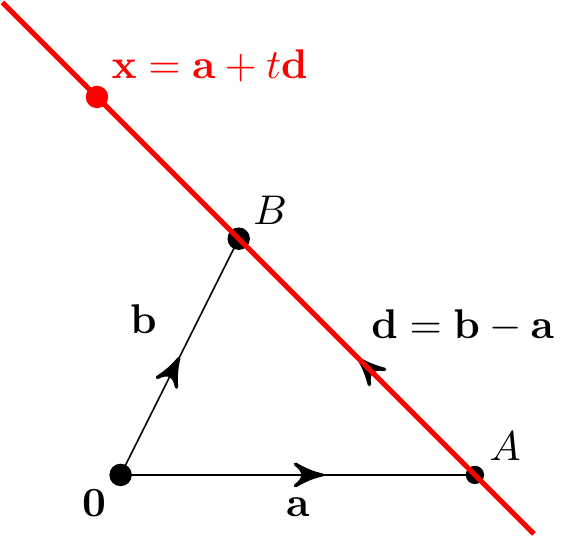
We can get to any point ${\bf x}$ on the line by travelling to $A$, then moving some distance in direction ${\bf d}$. In other words, \[ {\bf x} = {\bf a} + t{\bf d} \] for some real number $t$. This $t$ is a parameter and this equation for an arbitrary point ${\bf x}$ is called a parametric equation of the line.

It can useful to think of $t$ as a time variable. At $t=0$ we are at $A$, at $t=1$ we are at $B$ and we move at constant speed $|{\bf d}|$ along the line.

Note that there are many ways to write the line in parametric form. We could have started at $B$ rather than $A$, or indeed any other point on the line, and could use any non-zero multiple of ${\bf d}$ for the direction.

Example. $\,$ Find a parametric equation of the line joining $A=(1,2,1)$ and $B=(3,7,4)$.

The direction vector is \[ {\bf d} = {\bf b}-{\bf a} = \begin{pmatrix} 3\\7\\4 \end{pmatrix} - \begin{pmatrix} 1\\2\\1 \end{pmatrix} = \begin{pmatrix} 2\\5\\3 \end{pmatrix} \] so an arbitrary point on the line is $\displaystyle {\bf x} = {\bf a} + t{\bf d} = \begin{pmatrix} 1\\2\\1 \end{pmatrix} + t\begin{pmatrix} 2\\5\\3 \end{pmatrix}.$

Notice that if ${\bf x}$ has coordinates $x$, $y$, $z$, then we can eliminate $t$. \[ \begin{pmatrix} x\\y\\z \end{pmatrix}= \begin{pmatrix} a_1\\a_2\\a_3 \end{pmatrix} + t\begin{pmatrix} d_1\\d_2\\d_3 \end{pmatrix} \quad\implies \quad t = \frac{x-a_1}{d_1} = \frac{y-a_2}{d_2} = \frac{z-a_3}{d_3}. \] We say that $\;\;\displaystyle \frac{x-a_1}{d_1} = \frac{y-a_2}{d_2} = \frac{z-a_3}{d_3}\;\;$ are Cartesian equations of the line.

Notice if e.g. $d_1=0$, the above doesn’t quite work and we need to replace that equation by $x=a_1$. In fact, parametric form is often easier to work with in practice.

Example. $\,$ Find Cartesian equations of the line in the previous example. \[ {\bf x} = \begin{pmatrix} x\\y\\z \end{pmatrix} = \begin{pmatrix} 1 + 2t\\ 2 + 5t\\ 1 + 3t \end{pmatrix} \quad\implies\quad t = \frac{x-1}{2}=\frac{y-2}{5} = \frac{z-1}{3}, \] so Cartesian equations are $\displaystyle \frac{x-1}{2} = \frac{y-2}{5} = \frac{z-1}{3}$.

Example. $\,$ Suppose there are particles of mass $m_1$, $m_2$ at position vectors ${\bf R}_1$, ${\bf R}_2$ respectively. Where is the centre of mass ${\bf R}$? The definition of this is the weighted average position \[ {\bf R} = \frac{m_1{\bf R}_1 + m_2{\bf R}_2}{m_1+m_2}. \] We can rewrite this to show explicitly that it is a point on the line through ${\bf R}_1$ and ${\bf R}_2$ by adding and subtracting $m_2{\bf R}_1$ on the numerator: \[\begin{align*} {\bf R} &= \frac{(m_1 + m_2){\bf R}_1 + m_2({\bf R}_2-{\bf R}_1)}{m_1+m_2}\\ &= {\bf R}_1 + \frac{m_2}{m_1+m_2}({\bf R}_2-{\bf R}_1). \end{align*}\] This is the parametric equation of the line with ${\bf a}={\bf R}_1$ and ${\bf d}={\bf R}_2-{\bf R}_1$. It shows that ${\bf R}$ is a fraction $\displaystyle\frac{m_2}{m_1 + m_2}$ of the way along the line from ${\bf R}_1$ to ${\bf R}_2$.

Just to check, if $m_2=m_1$ then $\displaystyle\frac{m_2}{m_1+m_2} = \frac{m_1}{2m_1}=\frac12$, which is midway between, as expected. Similarly, if $m_1$ is much bigger than $m_2$ then $\displaystyle\frac{m_2}{m_1+m_2} \approx 0$, and if $m_1$ is much smaller than $m_2$ then $\displaystyle\frac{m_2}{m_1+m_2} \approx 1$.

If we had more particles, ${\bf R}_1,\ldots,{\bf R}_N$ with masses $m_1,\ldots,m_N$ then the corresponding centre of mass would be a similar weighted average \[ {\bf R} = \frac{m_1{\bf R}_1 + \ldots + m_N{\bf R}_N}{m_1 + \ldots + m_N}. \]

3.6 Planes in 3 dimensions

Now consider planes in three-dimensional space. One way to define a plane is by specifying any point ${\bf a}$ on it as well as a direction ${\bf n}$ which is orthogonal (perpendicular) to the plane. We call such a vector ${\bf n}$ a normal vector to the plane.

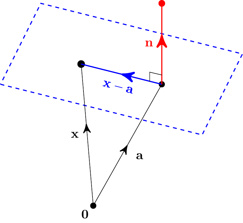
Then, given an arbitrary point on the plane with position vector ${\bf x}$, the vector ${\bf x}-{\bf a}$ is perpendicular to ${\bf n}$, so \[ ({\bf x}-{\bf a})\cdot{\bf n} = 0. \] This is a vector equation for the plane. There are lots of choices here: we could take any point on the plane and any non-zero multiple of the normal direction.

To find an equation for the plane involving the coordinates, \[ {\bf x} = \begin{pmatrix} x\\y\\z \end{pmatrix}, \quad {\bf a} = \begin{pmatrix} a_1\\a_2\\a_3 \end{pmatrix}, \quad {\bf n} = \begin{pmatrix} n_1\\n_2\\n_3 \end{pmatrix}, \] note that the vector equation gives ${\bf x}\cdot{\bf n} = {\bf a}\cdot{\bf n}$. We have \[ n_1x + n_2y + n_3z = n_1a_1 + n_2a_2 + n_3a_3. \] Or, since ${\bf a}$ and ${\bf n}$ are fixed, there is a constant $d$ with \[ n_1x + n_2y + n_3z = d. \] This is the standard form for the Cartesian equation of a plane.

Example. $\,$ Find a vector equation for the plane $x+2y+2z=1$.

We can read off the normal vector ${\bf n}=\begin{pmatrix} 1\\2\\2 \end{pmatrix}$ from the coefficients of $x$, $y$, $z$. We also need any point ${\bf a}$ on the plane. This must satisfy $a_1 + 2a_2 + 2a_3 = 1$, so a simple choice is $a_2=a_3=0$ and $a_1=1$. So a vector equation is \[ \left[\begin{pmatrix} x\\y\\z \end{pmatrix} - \begin{pmatrix} 1\\0\\0 \end{pmatrix}\right] \cdot \begin{pmatrix} 1\\2\\2 \end{pmatrix} =0. \]

Take any point ${\bf a}$ on a plane and any two non-zero, non-parallel vectors ${\bf u}$, ${\bf v}$ along the plane.

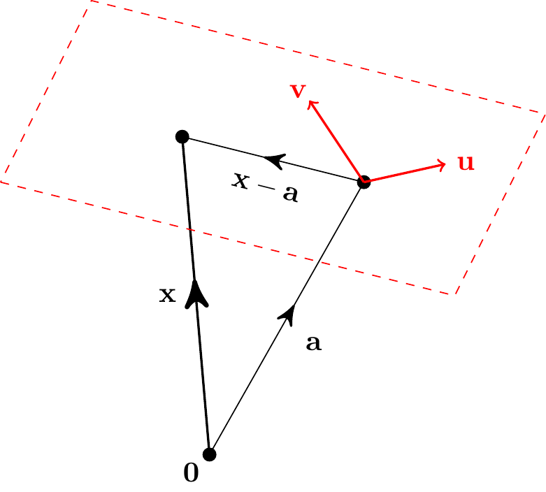
Then an arbitrary point on the plane can be written as \[ {\bf x} = {\bf a} + \lambda{\bf u} + \mu{\bf v} \] for some values of parameters $\lambda$ and $\mu$. This is a parametric equation for the plane.

Notice that if ${\bf n}$ is normal to the plane, then ${\bf n}$ is perpendicular to both ${\bf u}$ and ${\bf v}$. Hence \[ ({\bf x} - {\bf a})\cdot{\bf n} = \lambda{\bf u}\cdot{\bf n} + \mu{\bf v}\cdot{\bf n}=0 \] which is consistent with the vector equation of the plane.

Example. $\,$ From the earlier example we already found a point ${\bf a}=\begin{pmatrix} 1\\0\\0 \end{pmatrix}$ on this plane.

Now find two more points ${\bf b}$ and ${\bf c}$ on the plane with ${\bf a}$, ${\bf b}$ and ${\bf c}$ not all in a line. We can do this by e.g. fixing two of the coordinates to determine the third.

For example, ${\bf b}=\begin{pmatrix} -1 \\ 1 \\ 0 \end{pmatrix}$ and ${\bf c}=\begin{pmatrix} -1 \\ 0 \\ 1 \end{pmatrix}$ will work. Then \[ {\bf u}={\bf b}-{\bf a}=\begin{pmatrix} -2 \\ 1 \\ 0 \end{pmatrix} \quad\text{and}\quad {\bf v}={\bf c}-{\bf a}=\begin{pmatrix} -2 \\ 0 \\ 1 \end{pmatrix} \] give two non-parallel directions on the plane and a parametric equation is \[ {\bf x} = {\bf a} + \lambda{\bf u} + \mu{\bf v} = \begin{pmatrix} 1\\0\\0 \end{pmatrix} +\lambda\begin{pmatrix} -2\\1\\0 \end{pmatrix} + \mu\begin{pmatrix} -2\\0\\1 \end{pmatrix}. \] We could also get back to the Cartesian equation by setting ${\bf x}=\begin{pmatrix} x \\ y \\ z \end{pmatrix}= \begin{pmatrix} 1 - 2\lambda - 2\mu \\ \lambda \\ \mu \end{pmatrix}$ and eliminating $\lambda$ and $\mu$. Notice that this is a system of linear equations with two free parameters. So when solving a $3\times 3$ linear system via Gaussian elimination, if we find two free parameters, there is only one independent equation and the solutions must lie on a plane.

Now that we have various ways to write down planes, we can ask some further questions.

For instance, how can two planes intersect in 3 dimensional space? Either

they are equal (so they intersect everywhere),
they are parallel (so they do not intersect),
or they intersect in a straight line.

In this final case, notice that if the planes have normal vectors ${\bf n}_1$ and ${\bf n}_2$, then the angle between the planes is the same as the angle between these normal vectors:

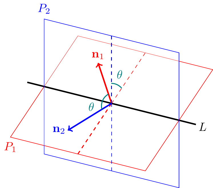
Example. $\,$ Find a parametric equation for the line of intersection of $x+2y+2z=1$ and $x+y+z=1$, and find the angle between the two planes.

The intersection solves the simultaneous equations \[ \begin{matrix} x + 2y + 2z = 1\\ x + y + z = 1 \end{matrix} \] Gaussian elimination gives \[ \left(\begin{matrix} 1 & 2 & 2 \\ 1 & 1 & 1 \end{matrix} \left|\,\begin{matrix} 1 \\ 1 \end{matrix}\right.\right) \xrightarrow{R_2 - R_1} \left(\begin{matrix} 1 & 2 & 2 \\ 0 & -1 & -1 \end{matrix} \left|\,\begin{matrix} 1 \\ 0 \end{matrix}\right.\right)\] \[\hspace{4.5cm} \xrightarrow{-R_2} \left(\begin{matrix} 1 & 2 & 2 \\ 0 & 1 & 1 \end{matrix} \left|\,\begin{matrix} 1 \\ 0\end{matrix}\right.\right) \] Taking $z=\lambda$ as a free parameter, back substitution gives $y=-\lambda$, $x=1$, so the intersection line has the parametric equation \[ {\bf x}=\begin{pmatrix} 1 \\ -\lambda \\ \lambda \end{pmatrix} =\begin{pmatrix} 1 \\ 0 \\ 0 \end{pmatrix} +\lambda\begin{pmatrix} 0 \\ -1 \\ 1 \end{pmatrix}. \] The normals to the two planes are \[ {\bf n}_1 = \begin{pmatrix} 1 \\ 2 \\ 2 \end{pmatrix} \quad\text{and}\quad {\bf n}_2 = \begin{pmatrix} 1 \\ 1 \\ 1 \end{pmatrix}, \] so the angle between the planes is the angle $\theta$ between these two vectors and satisfies \[ \cos\theta = \frac{{\bf n}_1\cdot{\bf n}_2}{|{\bf n}_1|\,|{\bf n}_2|} = \frac{1 + 2 + 2}{\sqrt{1^2 + 2^2 + 2^2}\sqrt{1^2 + 1^2 + 1^2}} = \frac{5}{3\sqrt{3}}. \]

Vector equations for planes also give us a quick way to find shortest distances between points and planes. Suppose we have a plane $({\bf x}-{\bf a})\cdot{\bf n}=0$. We can re-write this as \[ {\bf x}\cdot\hat{{\bf n}}={\bf a}\cdot\hat{{\bf n}}, \] where $\displaystyle\hat{{\bf n}}=\frac{{\bf n}}{|{\bf n}|}$ is a unit normal vector. The distance between ${\bf x}$ and the origin is $|{\bf x}|$ so, using the formula for scalar products, we see that \[ |{\bf x}|\,|\hat{{\bf n}}|\cos\theta = {\bf a}\cdot\hat{{\bf n}} \quad\implies\quad |{\bf x}| = \frac{{\bf a}\cdot\hat{{\bf n}}}{\cos\theta}, \] where $\theta$ is the angle between ${\bf x}$ and $\hat{{\bf n}}$. This distance is shortest when $\cos\theta=1$, i.e. when ${\bf x}$ is in the direction of ${\bf n}$, giving $|{\bf x}| = |{\bf a}\cdot\hat{{\bf n}}|$. Furthermore, the corresponding point on the plane is ${\bf x}=({\bf a}\cdot\hat{{\bf n}})\hat{{\bf n}}$ as this has the right length and direction.

Example. $\,$ Find the closest point to the origin on the plane $x+2y+2z=1$ and its distance from the origin.

We found ${\bf a}=\displaystyle\begin{pmatrix} 1 \\ 0 \\ 0 \end{pmatrix}$ and ${\bf n}=\displaystyle\begin{pmatrix} 1 \\ 2 \\ 2 \end{pmatrix}$ so a unit normal vector is $\hat{\bf n}=\dfrac13\begin{pmatrix} 1 \\ 2 \\ 2 \end{pmatrix}$.

The minimal distance is \[|{\bf a}\cdot\hat{\bf n}|=1\times\frac13+0\times\frac23+0\times\frac23=\frac13\] and the closest point is \[{\bf x}=\left({\bf a}\cdot\hat{\bf n}\right)\hat{\bf n}= \frac13\,\frac13\begin{pmatrix} 1 \\ 2 \\ 2 \end{pmatrix}= \frac19\begin{pmatrix} 1 \\ 2 \\ 2 \end{pmatrix}.\]

This can be generalised to find the shortest distance between an arbitrary point ${\bf b}$ and a plane by first translating everything so that ${\bf b}$ moves to the origin.

3.7 The Vector Product

There is another useful way to multiply two vectors in $\mathbb{R}^3$ which produces a vector. This is the vector product (also called the cross product) \[ {\bf u}\times{\bf v} = \begin{pmatrix} u_1\\u_2\\u_3 \end{pmatrix}\times \begin{pmatrix} v_1\\v_2\\v_3 \end{pmatrix} = \begin{pmatrix} u_2v_3 - u_3v_2\\ u_3v_1 - u_1v_3\\ u_1v_2 - u_2v_1 \end{pmatrix}. \] Note, this only works in 3-dimensional space $\mathbb{R}^3$.

A helpful way to remember the formula is to write it in terms of determinants: \[\begin{align*} {\bf u}\times{\bf v} = \begin{vmatrix} {\bf i} & {\bf j} & {\bf k} \\ u_1 & u_2 & u_3 \\ v_1 & v_2 & v_3 \end{vmatrix} &= {\bf i}\begin{vmatrix} u_2 & u_3 \\ v_2 & v_3 \end{vmatrix} -{\bf j}\begin{vmatrix} u_1 & u_3 \\ v_1 & v_3 \end{vmatrix} +{\bf k}\begin{vmatrix} u_1 & u_2 \\ v_1 & v_2 \end{vmatrix} \\ &= (u_2v_3 - u_3v_2){\bf i} + (u_3v_1 - u_1v_3){\bf j} + (u_1v_2 - u_2v_1){\bf k}. \end{align*}\]

Example. $\,$ Calculate ${\bf u}\times{\bf v}$ when ${\bf u}=\begin{pmatrix} 1 \\ 2 \\ 0 \end{pmatrix}$ and ${\bf v}=\begin{pmatrix} 2 \\ 3 \\ 1 \end{pmatrix}$.

We have \[ {\bf u}\times{\bf v} = \begin{pmatrix} 1 \\ 2 \\ 0 \end{pmatrix}\times \begin{pmatrix} 2 \\ 3 \\ 1 \end{pmatrix}= \begin{pmatrix} 2(1) - 0(3) \\ 0(2) - 1(1) \\ 1(3) - 2(1) \end{pmatrix}= \begin{pmatrix} 2 \\ -1 \\ -1 \end{pmatrix}. \]

Example. $\,$ Calculate ${\bf u}\times{\bf v}$ when ${\bf u}=\begin{pmatrix} a \\ 0 \\ 0 \end{pmatrix}$ and ${\bf v}=\begin{pmatrix} b\cos\theta \\ b\sin\theta \\ 0 \end{pmatrix}$.

Notice here that ${\bf u}$ and ${\bf v}$ lie in the $xy$-plane with an angle $\theta$ between them. We have \[ {\bf u}\times{\bf v} = \begin{pmatrix} a \\ 0 \\ 0 \end{pmatrix}\times \begin{pmatrix} b\cos\theta \\ b\sin\theta \\ 0 \end{pmatrix} = \begin{pmatrix} 0 \\ 0 \\ ab\sin\theta \end{pmatrix}. \] So ${\bf u}\times{\bf v}$ is in the $z$-direction and orthogonal (perpendicular) to both ${\bf u}$ and ${\bf v}$.

The vector product has the following properties:

Anti-commutativity: ${\bf u}\times{\bf v}=-{\bf v}\times{\bf u}$.
Scalar associativity: $(\lambda{\bf u})\times{\bf v} = \lambda({\bf u}\times{\bf v})$.
Distributivity: ${\bf u}\times({\bf v} + {\bf w}) = {\bf u}\times{\bf v} + {\bf u}\times{\bf w}$.

These are simple to show directly from the definition.

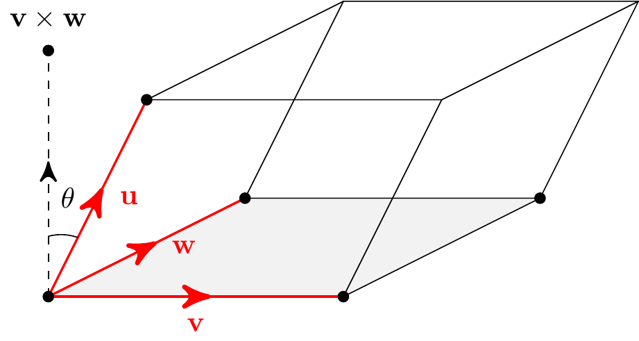
The geometrical interpretation of ${\bf u}\times{\bf v}$ is as a kind of ``directed area’’. Its direction is orthogonal to both ${\bf u}$ and ${\bf v}$ and its magnitude is the area of the parallelogram defined by ${\bf u}$ and ${\bf v}$, as shown here:

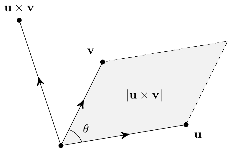
If $\theta$ is the angle between ${\bf u}$ and ${\bf v}$, then the area of the parallelogram is given by base times height, so \[ |{\bf u}\times{\bf v}| = |{\bf u}|\,|{\bf v}|\sin\theta. \]

This is a little complicated to prove in general from the definition of the vector product in terms of coordinates of ${\bf u}$ and ${\bf v}$, but we saw a specific case in the previous example.

Thus, just as the scalar product tells us when two non-zero vectors are perpendicular (it’s when ${\bf u}\cdot{\bf v}=0$), the vector product tells us when two non-zero vectors are parallel (it’s when ${\bf u}\times{\bf v}=\boldsymbol{0}$). In particular, ${\bf u}\times{\bf u}=\boldsymbol{0}$ for any vector ${\bf u}$.

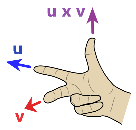
However, there are two directions orthogonal to the parallelogram. Should the vector ${\bf u}\times{\bf v}$ point up or down? This is determined by the right-hand rule – with your right hand, point your index finger in the ${\bf u}$ direction and your middle finger in the ${\bf v}$ direction. Then your thumb points in the ${\bf u}\times{\bf v}$ direction.

In particular, you can check that \[ {\bf i}\times{\bf j}={\bf k}, \quad {\bf j}\times{\bf k} = {\bf i}, \quad {\bf k}\times{\bf i} = {\bf j}, \] whereas \[ {\bf i}\times{\bf k} = -{\bf j},\quad {\bf j}\times{\bf i} = -{\bf k}, \quad {\bf k}\times{\bf j} = -{\bf i}. \]

We say that our usual Cartesian coordinates are right-handed because the standard basis vectors obey these identities.

The vector product gives us an easy way to find a vector perpendicular to two given vectors. We can use this to quickly find a normal vector to a plane.

Example. $\,$ Find a vector equation for the plane containing the three points \[A=(2,0,0),\qquad B=(0,4,0), \qquad C=(0,0,-3).\]

We can create two independent directions on the plane using the three points: \[ {\bf u} = \overrightarrow{AB} = \begin{pmatrix} 0 \\ 4 \\ 0 \end{pmatrix} - \begin{pmatrix} 2 \\ 0 \\ 0 \end{pmatrix} = \begin{pmatrix} -2 \\ 4 \\ 0 \end{pmatrix}\] \[ {\bf v} = \overrightarrow{AC} = \begin{pmatrix} 0 \\ 0 \\ -3 \end{pmatrix} - \begin{pmatrix} 2 \\ 0 \\ 0 \end{pmatrix} = \begin{pmatrix} -2 \\ 0 \\ -3 \end{pmatrix}. \] Then a normal vector to the plane is \[ {\bf n} = {\bf u}\times{\bf v} = \begin{pmatrix} -2\\4\\0 \end{pmatrix} \times \begin{pmatrix} -2\\0\\-3 \end{pmatrix} = \begin{pmatrix} -12\\-6\\8 \end{pmatrix}. \] Now we just need any point e.g. ${\bf a} = \begin{pmatrix} 2 \\ 0 \\ 0 \end{pmatrix}$ on the plane and we then have a vector equation $({\bf x}-{\bf a})\cdot{\bf n}=0$.

We can also use the vector product to find a vector equation of a line. Recall the parametric equation of a line – if ${\bf a}$ is a point on the line and ${\bf d}$ is its direction, then \[ {\bf x} = {\bf a} + t{\bf d} \quad \implies {\bf x} - {\bf a} = t{\bf d}. \] Taking the cross product with ${\bf d}$, and using ${\bf d}\times{\bf d}=\boldsymbol{0}$, gives a vector equation of the line, \[ ({\bf x}-{\bf a})\times{\bf d} = \boldsymbol{0}. \]

Example. $\,$ Find a vector equation for the line parallel to ${\bf i}+2{\bf j}-{\bf k}$ which passes through the point $(0,1,0)$.

The line has direction ${\bf d}={\bf i} +2{\bf j} - {\bf k}$ and a point on the line is ${\bf a}={\bf j}$ so the vector equation is $({\bf x}-{\bf a})\times{\bf d}=\boldsymbol{0}$, that is, \[\begin{align*} ({\bf x}-{\bf a})\times{\bf d} &= \begin{pmatrix} x \\ y-1 \\ z \end{pmatrix}\times \begin{pmatrix} 1 \\ 2 \\ -1 \end{pmatrix} =\begin{pmatrix} 0 \\ 0 \\ 0 \end{pmatrix}\\ &\implies\quad \begin{pmatrix} 1 - y - 2z \\ x + z \\ 2x - y + 1 \end{pmatrix}= \begin{pmatrix} 0 \\ 0 \\ 0 \end{pmatrix}. \end{align*}\] The equations of each of the the coordinates here give us Cartesian equations for the line and solving these equations simultaneously with one variable as a parameter would get us back to the parametric form.

We now have Cartesian, parametric and vector equations for both lines and planes in 3 dimensions. Being able to describe the same object in different ways gives us extra mathematical flexibility.

3.8 Distances Between Lines

Finding the shortest distance between two lines is another application of vector products.

First, suppose the two lines are parallel. Thus they have the same direction vector ${\bf u}$ and can be written in parametric form as \[\begin{align*} {\bf x} &= {\bf a} + \lambda{\bf u},\\ {\bf x} &= {\bf b} + \mu{\bf u} \end{align*}\] for some vectors ${\bf a}$ and ${\bf b}$.

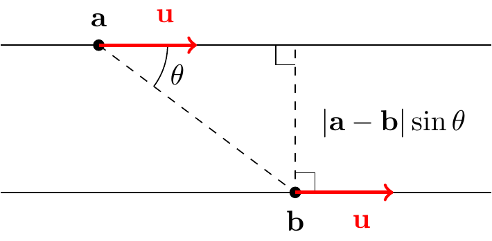
The shortest distance will be the length of the line perpendicular to both lines as shown. If $\theta$ is the angle between ${\bf a}-{\bf b}$ and ${\bf u}$, then this distance is $|{\bf a}-{\bf b}|\sin\theta$. However, \[ \big|({\bf a}-{\bf b})\times{\bf u}\big| = |{\bf a}-{\bf b}|\,|{\bf u}|\sin\theta \] so the distance can be written $\big|({\bf a}-{\bf b})\times\hat{{\bf u}}\big|$, where $\hat{{\bf u}} = {\bf u}/|{\bf u}|$.

Example. $\,$ Find the distance between the lines with Cartesian equations \[ \frac{x-3}{2} = \frac{y+8}{-2} = \frac{z-1}{1} \quad\text{and}\quad \frac{x+5}{4} = \frac{y+3}{-4} = \frac{z-6}{2}. \]

The direction vectors ${\bf u}=\begin{pmatrix} 2 \\ -2 \\ 1 \end{pmatrix}$ and ${\bf v}=\begin{pmatrix} 4 \\ -4 \\ 2 \end{pmatrix}$ are parallel since ${\bf v}=2{\bf u}$.

A unit vector in this direction is $\hat{{\bf u}} = \dfrac13\begin{pmatrix} 2 \\ -2 \\ 1 \end{pmatrix}$, and points on the two lines are ${\bf a}=\begin{pmatrix} 3 \\ -8 \\ 1 \end{pmatrix}$ and ${\bf b}=\begin{pmatrix} -5 \\ -3 \\ 6 \end{pmatrix}$ respectively. So \[\begin{align*} ({\bf a}-{\bf b})\times\hat{{\bf u}} &= \frac13\begin{pmatrix} 8 \\ -5 \\ -5 \end{pmatrix}\times \begin{pmatrix} 2 \\ -2 \\ 1 \end{pmatrix} \\ &= \frac13\begin{pmatrix} -5-10 \\ -10-8 \\ -16+10 \end{pmatrix}= \frac13\begin{pmatrix} -15 \\ -18 \\ -6 \end{pmatrix} =\begin{pmatrix} -5 \\ -6 \\ -2 \end{pmatrix}. \end{align*}\] The minimum distance is then the length of this, that is, $\sqrt{5^2+6^2+2^2}=\sqrt{65}$.

Now consider the case where the two lines are parallel. Then we can write arbitrary points on the two lines as \[\begin{align*} {\bf x}_1 &= {\bf a} + \lambda{\bf u},\\ {\bf x}_2 &= {\bf b} + \mu{\bf v} \end{align*}\] for some vectors ${\bf a}$, ${\bf b}$ and non-parallel direction vectors ${\bf u}$, ${\bf v}$.

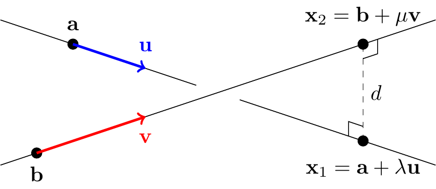
The distance is minimum when the line connecting ${\bf x}_1$ to ${\bf x}_2$ is perpendicular to the two lines, hence to both ${\bf u}$ and ${\bf v}$. But we know a vector in this direction, namely ${\bf n}={\bf u}\times{\bf v}$. In fact, if $d$ denotes the minimum distance, then letting $\hat{{\bf n}}={\bf n}/|{\bf n}|$, we must have \[ {\bf x}_1-{\bf x}_2 = \pm d\hat{{\bf n}} \] and so \[ ({\bf a} + \lambda{\bf u}) - ({\bf b} + \mu{\bf v}) = \pm d\hat{{\bf n}}. \] Taking the scalar product of both sides with $\hat{{\bf n}}$, and remembering ${\bf u}\cdot\hat{{\bf n}}={\bf v}\cdot\hat{{\bf n}} = 0$ and $\hat{{\bf n}}\cdot\hat{{\bf n}}=1$, we obtain \[ ({\bf a} -{\bf b})\cdot\hat{{\bf n}} = \pm d. \] In other words, the minimum distance between the two lines is \[ d = \big|({\bf a}-{\bf b})\cdot\hat{{\bf n}}\big| = \left|({\bf a}-{\bf b})\cdot\frac{{\bf u}\times{\bf v}}{|{\bf u}\times{\bf v}|}\right|. \]

Example. $\,$ Find the distance between the lines given by parametric equations \[ {\bf x} = \begin{pmatrix} 1 \\ 1 \\ 0 \end{pmatrix} + \lambda\begin{pmatrix} 1 \\ 6 \\ 2 \end{pmatrix} \quad\text{and}\quad {\bf x}=\begin{pmatrix} 1 \\ 5 \\ -2 \end{pmatrix} + \mu\begin{pmatrix} 2 \\ 15 \\ 6 \end{pmatrix}. \] The lines are not parallel since their direction vectors ${\bf u}=\begin{pmatrix} 1 \\ 6 \\ 2 \end{pmatrix}$ and ${\bf v}=\begin{pmatrix} 2 \\ 15 \\ 6 \end{pmatrix}$ aren’t multiples of each other. A vector perpendicular to both is \[ {\bf n} = {\bf u}\times{\bf v} = \begin{pmatrix} 1 \\ 6 \\ 2 \end{pmatrix}\times \begin{pmatrix} 2 \\ 15 \\ 6 \end{pmatrix} = \begin{pmatrix} 36-30 \\ 4-6 \\ 15-12 \end{pmatrix} = \begin{pmatrix} 6 \\ -2 \\ 3 \end{pmatrix}. \] This has length $|{\bf n}|=\sqrt{6^2 + (-2)^2 + 3^2} = 7$ so the unit vector in this direction is \[ \hat{{\bf n}} = \frac17\begin{pmatrix} 6 \\ -2 \\ 3 \end{pmatrix}. \] Taking points on the lines ${\bf a}=\begin{pmatrix} 1 \\ 1 \\ 0 \end{pmatrix}$ and ${\bf b}=\begin{pmatrix} 1 \\ 5 \\ -2 \end{pmatrix}$, we have \[ ({\bf a}-{\bf b})\cdot\hat{{\bf n}} = \begin{pmatrix} 0 \\ -4 \\ 2 \end{pmatrix}\cdot \frac17\begin{pmatrix} 6 \\ -2 \\ 3 \end{pmatrix} = \frac17(0+8+6) = 2 \] and so the minimum distance is $2$.

3.9 The Scalar Triple Product

Given three vectors ${\bf u}$, ${\bf v}$, ${\bf w}$ in $\mathbb{R}^3$, the scalar triple product is \[{\bf u}\cdot({\bf v}\times{\bf w}).\] Geometrically, this gives the volume of the parallelepiped (the 3-d version of a parallelogram) with edges given by ${\bf u}$, ${\bf v}$ and ${\bf w}$.

To see why this is, note that the volume is the area of the base times the height. We know that the area of the base is $|{\bf v}\times{\bf w}|$. The vector ${\bf n}={\bf v}\times{\bf w}$ is normal to the base. If it makes an angle $\theta$ with ${\bf u}$ then the height of the parallelepiped is $|{\bf u}|\cos\theta$. So the volume is \[ |{\bf v}\times{\bf w}|\,|{\bf u}|\cos\theta = {\bf u}\cdot({\bf v}\times{\bf w}). \]

Notice that cycling ${\bf u}$, ${\bf v}$, ${\bf w}$ doesn’t change the volume, so \[ {\bf u}\cdot({\bf v}\times{\bf w}) = {\bf v}\cdot({\bf w}\times{\bf u}) = {\bf w}\cdot({\bf u}\times{\bf v}). \]

On the other hand, by the anti-commutativity of the vector product, \[ {\bf u}\cdot({\bf v}\times{\bf w}) = -{\bf u}\cdot({\bf w}\times{\bf v}) = -{\bf v}\cdot({\bf u}\times{\bf w}) = -{\bf w}\cdot({\bf v}\times{\bf u}). \]

Also notice that if ${\bf u}={\bf v}$ or ${\bf u}={\bf w}$, then the volume is zero so \[ {\bf v}\cdot({\bf v}\times{\bf w}) = {\bf w}\cdot({\bf v}\times{\bf w}) = 0. \] This again tells us that ${\bf v}\times{\bf w}$ is perpendicular to both ${\bf v}$ and ${\bf w}$.

In terms of determinants, the scalar triple product has a nice expression: \[\begin{align*} {\bf u}\cdot({\bf v}\times{\bf w}) &= (u_1{\bf i} + u_2{\bf j} + u_3{\bf k})\cdot \begin{vmatrix} {\bf i} & {\bf j} & {\bf k}\\ v_1 & v_2 & v_3\\ w_1 & w_2 & w_3 \end{vmatrix} \\ &= \begin{vmatrix} u_1 & u_2 & u_3\\ v_1 & v_2 & v_3\\ w_1 & w_2 & w_3 \end{vmatrix}. \end{align*}\]

3.10 Application to Mechanics

Suppose we have a position vector ${\bf r}(t)$ which depends on time $t$. Then we can differentiate ${\bf r}(t)$ to give derivative \[ \dot{{\bf r}}(t) = \frac{d{\bf r}}{dt} = \lim_{h\to 0} \frac{{\bf r}(t+h) - {\bf r}(t)}{h}. \]

In Physics,we often put a dot over a variable as shorthand for differentiation with respect to time.
We will look more at the limit definition of differentiation next term.

To calculate this derivative, we just differentiate each component separately: \[ {\bf r}(t) = \begin{pmatrix} x(t) \\ y(t) \\ z(t) \end{pmatrix} \quad\implies\quad \dot{{\bf r}}(t) = \begin{pmatrix} \dot{x}(t)\\ \dot{y}(t)\\ \dot{z}(t) \end{pmatrix}. \]

Differentiating vectors like this satisfies a number of natural properties which can be checked directly from the definitions and the product rule. For vector-valued functions ${\bf r}(t)$, ${\bf s}(t)$ and a scalar $\lambda(t)$ all depending on $t$, we have: \[ \dfrac{d}{dt}({\bf r} + {\bf s}) =\dot{{\bf r}} + \dot{{\bf s}}, \qquad \dfrac{d}{dt}(\lambda{\bf r}) =\dot{\lambda}{\bf r} + \lambda\dot{{\bf r}}, \] \[ \dfrac{d}{dt}({\bf r}\cdot{\bf s})= \dot{{\bf r}}\cdot{\bf s} + {\bf r}\cdot\dot{{\bf s}}, \qquad \dfrac{d}{dt}({\bf r}\times{\bf s})= \dot{{\bf r}}\times{\bf s} + {\bf r}\times\dot{{\bf s}}.\]

In the last formula it’s important not to change the order of the ${\bf r}$ and ${\bf s}$, since the vector product depends on the order and ${\bf u}\times{\bf v}=-{\bf v}\times{\bf u}$.

In mechanics, we can use this to find vector expressions for various quantities associated with a particle of mass $m$ and position vector ${\bf r}(t)$:

Velocity: ${\bf v} = \dot{{\bf r}}$.
Momentum: ${\bf p} = m{\bf v} = m\dot{{\bf r}}$.
Acceleration: ${\bf a} = \dot{{\bf v}} = \ddot{{\bf r}}$.
Force (Newton’s Second Law): ${\bf F} = m{\bf a} = \dot{{\bf p}} = m\ddot{{\bf r}}$.
Angular momentum about the origin: ${\bf L} = {\bf r}\times{\bf p} = m{\bf r}\times\dot{{\bf r}}$.
Moment of force about the origin (torque): $\boldsymbol{\tau} = {\bf r}\times{\bf F} = m{\bf r}\times\ddot{{\bf r}}$.

Newton’s Second Law tells us that if ${\bf F}=\boldsymbol{0}$ then $\dot{{\bf p}}=\boldsymbol{0}$, so ${\bf p}$ is constant. In other words, if the net force on an object is continually zero then the momentum is conserved.

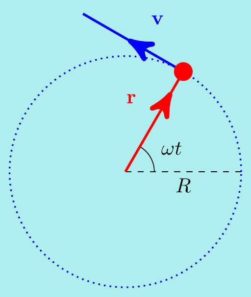
Example. $\,$ A particle moves with position vector \[ {\bf r}(t) = \begin{pmatrix} x(t) \\ y(t) \\ 0 \end{pmatrix} = \begin{pmatrix} R\cos(\omega t) \\ R\sin(\omega t) \\ 0 \end{pmatrix} \] for some constants $R$ and $\omega$. Show that the particle moves in a circle, find the force acting on the particle, and show its angular momentum is conserved.

Since $x(t)^2 + y(t)^2 = R^2$, we see that the particle moves around a circle in the $xy$-plane with radius $R$ centred at the origin. To find the force ${\bf F}$, we first calculate the velocity: \[ {\bf v} = \begin{pmatrix} \dot{x}\\ \dot{y}\\ 0 \end{pmatrix} = \begin{pmatrix} -R\omega \sin(\omega t)\\ R\omega\cos(\omega t)\\0 \end{pmatrix}. \] Notice that ${\bf r}\cdot{\bf v}=0$ at any time $t$ so the velocity is always perpendicular to the position, meaning along the tangent to the circle:

The acceleration is ${\bf a} = \dot{{\bf v}} = \begin{pmatrix} -R\omega^2\cos(\omega t)\\ -R\omega^2\sin(\omega t)\\ 0 \end{pmatrix} = -\omega^2{\bf r}$.

Hence the force is ${\bf F}=m{\bf a} = -m\omega^2{\bf r}$. Notice that this is always directed towards the origin. Also, the angular momentum is \[\begin{align*} {\bf L} &= m{\bf r}(t)\times{\bf v}(t)\\ &= m\begin{pmatrix} R\cos(\omega t)\\ R\sin(\omega t)\\ 0 \end{pmatrix}\times \begin{pmatrix} -R\omega\sin(\omega t)\\ R\omega\cos(\omega t)\\ 0 \end{pmatrix}\\ &= mR^2\omega\Big(\cos^2(\omega t) + \sin^2(\omega t)\Big){\bf k}\\ &= mR^2\omega{\bf k}. \end{align*}\] This is independent of $t$, so the angular momentum ${\bf L}$ is conserved.

More generally, differentiating ${\bf L}=m{\bf r}\times\dot{{\bf r}}$ gives \[\begin{align*} \dot{{\bf L}} &= m\dot{{\bf r}}\times\dot{{\bf r}} + m{\bf r}\times\ddot{{\bf r}}\\ &= \boldsymbol{0} + {\bf r}\times{\bf F}\\ &= \boldsymbol{\tau}, \end{align*}\] so the rate of change of angular momentum is equal to the torque (“turning force”) on the particle.

If the force always acts directly toward the origin, then we call it a central force. (Think about e.g. gravitational attraction.)
Under such a force, we have $\boldsymbol{\tau}={\bf r}\times{\bf F}=\boldsymbol{0}$, as ${\bf r}$ and ${\bf F}$ are parallel. Hence $\dot{{\bf L}}=\boldsymbol{0}$ and this means angular momentum is conserved.

We can also see that the angular momentum only arises from the perpendicular component of the velocity by decomposing the velocity as ${\bf v} = {\bf v}_\parallel + {\bf v}_\perp$, where ${\bf v}_\parallel$ is parallel to the position vector ${\bf r}$ and ${\bf v}_\perp$ is perpendicular to ${\bf r}$:

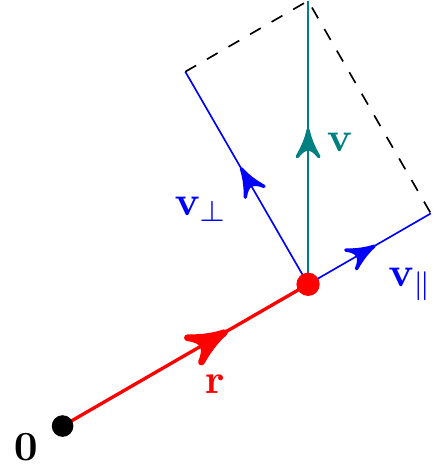
Then \[\begin{align*} {\bf L} = m{\bf r}\times{\bf v}_\parallel + m{\bf r}\times{\bf v}_\perp = \boldsymbol{0} + m{\bf r}\times{\bf v}_\perp = m{\bf r}\times{\bf v}_\perp. \end{align*}\] which doesn’t depend on ${\bf v}_\parallel$.

3.11 Eigenvalues and eigenvectors

Multiplying a vector in $\mathbb{R}^n$ by an $n\times n$ matrix $A$ changes it into another vector – for example, \[ \begin{pmatrix} 2 \\ 3 \end{pmatrix}\longmapsto \begin{pmatrix} 2 & 2 \\ 0 & 4 \end{pmatrix} \begin{pmatrix} 2 \\ 3 \end{pmatrix} = \begin{pmatrix} 10 \\ 12 \end{pmatrix}. \] So we can think of matrices as representing transformations of space, mapping vectors to vectors. These are called linear maps and they “respect linear things”. For instance, they map straight lines to straight lines, maybe by stretching, reflecting or rotating space. Transformations like this will often have “preferred” directions, such as the location of a reflecting mirror or the axis of a rotation. These special directions are examples of eigenvectors belonging to a matrix, and finding them can make difficult linear algebra problems easy. They have many applications that you will learn about in this and later courses.

Example.

(1)$\;\;$ The matrix $A=\begin{pmatrix} 2 & 0 \\ 0 & 4 \end{pmatrix}$ stretches vectors: $\;\;\begin{pmatrix} x \\ y \end{pmatrix}\longmapsto \begin{pmatrix} 2 & 0 \\ 0 & 4 \end{pmatrix}\begin{pmatrix} x \\ y \end{pmatrix} =\begin{pmatrix} 2x \\ 4y \end{pmatrix}$.

If ${\bf v}=\begin{pmatrix} t \\ 0 \end{pmatrix}$ then $A{\bf v}=2{\bf v}$. It stretches vectors on the $x$-axis by factor 2 but doesn’t change their direction.
If ${\bf v}=\begin{pmatrix} 0 \\ t \end{pmatrix}$ then $A{\bf v}=4{\bf v}$. It stretches vectors on the $y$-axis by factor 4 but doesn’t change their direction.
All other vectors change direction: $A{\bf v}$ is not a multiple of ${\bf v}$.

(2)$\;\;$ The matrix $A=\begin{pmatrix} 0 & 1 \\ 1 & 0 \end{pmatrix}$ reflects in the line $y=x$: $\;\;\begin{pmatrix} x \\ y \end{pmatrix}\longmapsto \begin{pmatrix} 0 & 1 \\ 1 & 0 \end{pmatrix}\begin{pmatrix} x \\ y \end{pmatrix} =\begin{pmatrix} y \\ x \end{pmatrix}$.

If ${\bf v}=\begin{pmatrix} t \\ t \end{pmatrix}$ then $A{\bf v}={\bf v}$. It doesn’t change these vectors - they lie on the mirror.
If ${\bf v}=\begin{pmatrix} t \\ -t \end{pmatrix}$ then $A{\bf v}=-{\bf v}$. These are vectors perpendicular to the mirror.
All other vectors change direction when reflected: $A{\bf v}$ is not a multiple of ${\bf v}$.

Suppose $A$ is an $n\times n$ matrix and \[ A{\bf v} = \lambda{\bf v} \] for some scalar $\lambda$ and some non-zero vector ${\bf v}\neq\boldsymbol{0}$. Then we say that $\lambda$ is an eigenvalue of $A$ and ${\bf v}$ is an eigenvector corresponding to $\lambda$.

The prefix “eigen-” comes from the German for “own”, “special” or “characteristic”. They are special values and vectors associated with a particular matrix.}

We can actually find what the eigenvalues must be without mentioning the eigenvectors. Rearrange the above equation \[\begin{align*} A{\bf v} = \lambda{\bf v} \iff A{\bf v} - \lambda{\bf v} = \boldsymbol{0} \iff (A-\lambda I){\bf v} = \boldsymbol{0} \end{align*}\] where $I=I_n$ is the $n\times n$ identity matrix. Notice that ${\bf v}=\boldsymbol{0}$ is automatically a solution to the system \[(A-\lambda I){\bf v}=\boldsymbol{0}.\] If there is also a non-zero solution ${\bf v} \neq \boldsymbol{0}$, then this system doesn’t have a unique solution. In particular, $\lambda$ is an eigenvalue of $A$ precisely when \[\det(A - \lambda I) = 0.\] Because of the way determinants are defined, $\det(A - \lambda I)$ is a polynomial in $\lambda$ of degree $n$ and is called the characteristic polynomial of $A$.

Once we have found the roots of the characteristic polynomial to find the eigenvalues $\lambda$, we can then solve the linear system $(A-\lambda I){\bf v}=\boldsymbol{0}$ to find the corresponding eigenvectors for each $\lambda$ in turn. Because the system is singular, we know the ${\bf v}$ for each eigenvalue are not unique, so it is convenient to express them in terms of the eigenspace $V_\lambda$. This is the set spanned by the possible ${\bf v}$ corresponding to $\lambda$, together with the zero vector.

It’s easiest to see how this works with an example.

Example. Find the eigenvalues and corresponding eigenspaces of $A=\begin{pmatrix} 2 & 2 \\ 0 & 4 \end{pmatrix}.$

Find the eigenvalues: these are the roots of the characteristic polynomial \[ \det(A - \lambda I) = \begin{vmatrix} 2-\lambda & 2 \\ 0 & 4-\lambda \end{vmatrix} =0 \quad\iff\quad (2-\lambda)(4-\lambda) = 0. \] So the eigenvalues are $\lambda=2$ and $4$.

Find the eigenspace $V_2$: the eigenvectors ${\bf v}$ for $\lambda=2$ satisfy $(A-2I){\bf v}=\boldsymbol{0}$ (which we remember has infinitely many solutions).

Writing ${\bf v}=\begin{pmatrix} x \\ y \end{pmatrix}$, we have $\begin{pmatrix} 0 & 2 \\ 0 & 2 \end{pmatrix} \begin{pmatrix} x \\ y \end{pmatrix} = \begin{pmatrix} 2y \\ 2y \end{pmatrix} = \begin{pmatrix} 0 \\ 0 \end{pmatrix}$ and thus $y=0$ and $x=\mu$ for a parameter $\mu.$ The eigenvectors are thus ${\bf v} = \begin{pmatrix} \mu \\ 0 \end{pmatrix}= \mu\begin{pmatrix} 1 \\ 0 \end{pmatrix}$ for $\mu\neq 0$.

This eigenspace consists of all eigenvectors as well as the zero vector, i.e. $V_2 = \operatorname{Span}\left\{\begin{pmatrix} 1 \\ 0 \end{pmatrix}\right\}$.

Find the eigenspace $V_4$: the eigenvectors ${\bf v}$ satisfy the linear system $(A-4I){\bf v}=\boldsymbol{0}$, or \[ \begin{pmatrix} -2 & 2 \\ 0 & 0 \end{pmatrix} \begin{pmatrix} x \\ y \end{pmatrix} = \begin{pmatrix} -2x + 2y \\ 0 \end{pmatrix} = \begin{pmatrix} 0 \\ 0 \end{pmatrix} \quad\implies\quad y=\mu, x=\mu. \] So ${\bf v}=\begin{pmatrix} \mu\\ \mu \end{pmatrix} = \mu\begin{pmatrix} 1 \\ 1 \end{pmatrix}$ for $\mu\neq 0$, and this eigenspace is $V_4 = \operatorname{Span}\left\{\begin{pmatrix} 1 \\ 1 \end{pmatrix}\right\}$.

Just for fun, let’s look at the interpretation of the previous example as a transformation.

The matrix $A=\begin{pmatrix} 2 & 2 \\ 0 & 4 \end{pmatrix}$ maps $\begin{pmatrix} x \\ y \end{pmatrix}\longmapsto \begin{pmatrix} 2 & 2 \\ 0 & 4 \end{pmatrix} \begin{pmatrix} x \\ y \end{pmatrix} = \begin{pmatrix} 2x + 2y \\ 4y \end{pmatrix}$.

This has the effect of stretching and shearing an initial square region into a parallelogram:

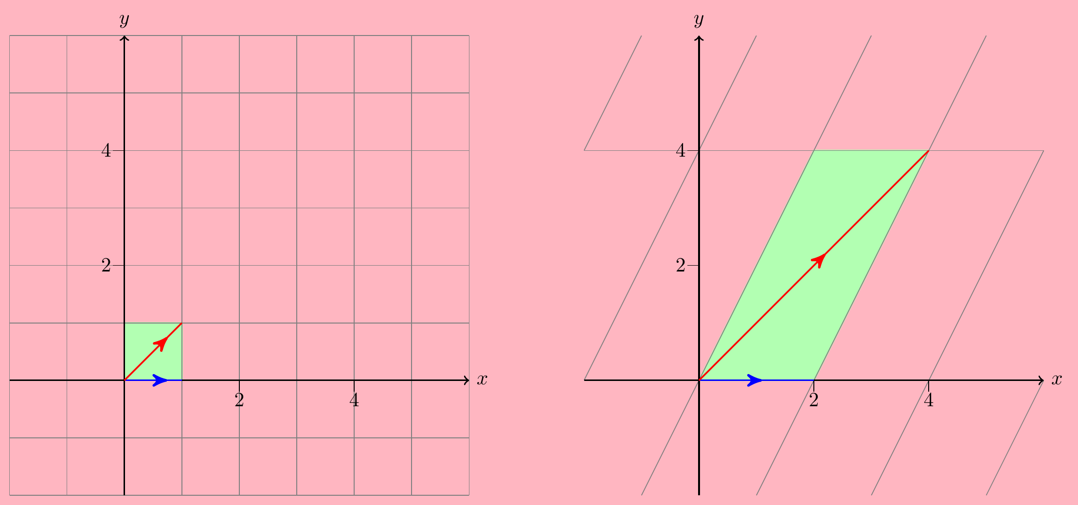
Notice that straight lines are mapped to straight lines – this is always true when you multiply by a (non-singular) matrix. The blue and red arrows in the left hand plot show the eigenvectors $\begin{pmatrix} 1 \\ 0 \end{pmatrix}$ and $\begin{pmatrix} 1 \\ 1 \end{pmatrix}$. They are stretched in length by their corresponding eigenvalues $2$ and $4$, but they don’t change direction. Any straight line that is not parallel to one of these eigenvectors will necessarily change its direction – like the vertical lines, for instance.

Another fun fact: the determinant of $A$ tells you how much the area of the square is increased during its transformation, so in this example, the square with area $1$ becomes a parallelogram with area $\det(A)=8$. A negative determinant would mean that there is also a reflection involved, leading to a “negative area”.

Example. $\,$ Find the eigenvalues and eigenspaces of the matrix $A = \begin{pmatrix} 5 & 6 & -3\\ 0 & -1 & 0\\ 6 & 6 & -4 \end{pmatrix}$.

Find the eigenvalues: The characteristic polynomial is $\det(A-\lambda I_3)=0$, and \[\begin{align*} \det(A-\lambda I_3) &= \begin{vmatrix} 5-\lambda & 6 & -3 \\ 0 & -1-\lambda & 0 \\ 6 & 6 & -4-\lambda \end{vmatrix} \\ &\overset{\scriptstyle transp.}{=} \begin{vmatrix} 5-\lambda & 0 & 6 \\ 6 & -1-\lambda & 6 \\ -3 & 0 & -4-\lambda \end{vmatrix} \\ &= (5-\lambda)\begin{vmatrix} -1-\lambda & 6 \\ 0 & -4-\lambda \end{vmatrix} +6\begin{vmatrix} 6 & -1-\lambda \\ -3 & 0 \end{vmatrix} \\ &= (5-\lambda)(1+\lambda)(4+\lambda) - 18(1+\lambda)\\ &= (1+\lambda)(20 + \lambda - \lambda^2 - 18) \\ &= (1+\lambda)^2(2-\lambda). \end{align*}\] So we have eigenvalues $\lambda=-1,-1, 2$.

Find the eigenspace $V_{-1}$: eigenvectors ${\bf v}$ corresponding to $\lambda=-1$ satisfy $(A+I){\bf v}=\boldsymbol{0}$, i.e. \[\begin{align*} \begin{pmatrix} 6 & 6 & -3 \\ 0 & 0 & 0 \\ 6 & 6 & -3 \end{pmatrix} \begin{pmatrix} x \\ y \\ z \end{pmatrix} = \begin{pmatrix} 0 \\ 0 \\ 0 \end{pmatrix}. \end{align*}\] There is effectively only one equation $2x + 2y -z = 0$, so there will be a two-parameter family of solutions (i.e. it’s a plane). Choosing $x=\mu$ and $y=\nu$ shows that \[ {\bf v} = \begin{pmatrix} x \\ y \\ z \end{pmatrix} = \begin{pmatrix} \mu \\ \nu \\ 2\mu + 2\nu \end{pmatrix} = \mu\begin{pmatrix} 1 \\ 0 \\ 2 \end{pmatrix} + \nu\begin{pmatrix} 0 \\ 1 \\ 2 \end{pmatrix} \] and so \[ V_{-1} = \operatorname{Span}\left\{\begin{pmatrix} 1 \\ 0 \\ 2 \end{pmatrix}, \begin{pmatrix} 0 \\ 1 \\ 2\end{pmatrix}\right\}. \]

Find the eigenspace $V_2$: eigenvectors ${\bf v}$ corresponding to $\lambda=2$ satisfy $(A-2I){\bf v}=\boldsymbol{0}$, i.e. \[ \begin{pmatrix} 3 & 6 & -3 \\ 0 & -3 & 0 \\ 6 & 6 & -6 \end{pmatrix} \begin{pmatrix} x \\ y \\ z \end{pmatrix} = \begin{pmatrix} 0 \\ 0 \\ 0 \end{pmatrix}. \] This time we can’t immediately read off the solutions so easily, so instead let’s solve by Gaussian elimination: \[ \left(\begin{matrix} 3 & 6 & -3 \\ 0 & -3 & 0 \\ 6 & 6 & -6 \end{matrix} \left|\,\begin{matrix} 0 \\ 0 \\ 0 \end{matrix}\right.\right) \xrightarrow[\frac13R_3]{\frac13R_1\;,\;-\frac13R_2} \left(\begin{matrix} 1 & 2 & -1 \\ 0 & 1 & 0 \\ 1 & 1 & -1 \end{matrix} \left|\,\begin{matrix} 0 \\ 0 \\ 0 \end{matrix}\right.\right) \] \[\qquad\qquad\xrightarrow[R_3-R_2]{R_1-2R_2} \left(\begin{matrix} 1 & 0 & -1 \\ 0 & 1 & 0 \\ 1 & 0 & -1 \end{matrix} \left|\,\begin{matrix} 0 \\ 0 \\ 0 \end{matrix}\right.\right) \xrightarrow{-\tfrac13R_2} \left(\begin{matrix} 1 & 0 & -1 \\ 0 & 1 & 0 \\ 0 & 0 & 0 \end{matrix} \left|\,\begin{matrix} 0 \\ 0 \\ 0 \end{matrix}\right.\right)\] Hence $y=0$ and taking $z=\mu$ to be a free parameter, we get $x=\mu$. So \[ {\bf v} = \begin{pmatrix} \mu \\ 0 \\ \mu \end{pmatrix} = \mu\begin{pmatrix} 1 \\ 0 \\ 1 \end{pmatrix} \quad\text{and so}\quad V_2 = \operatorname{Span}\left\{\begin{pmatrix} 1 \\ 0 \\ 1 \end{pmatrix}\right\}. \]

Notice in the above two examples that the combined eigenspaces spanned the whole of space ($\mathbb{R}^2$ in the first case and $\mathbb{R}^3$ in the second). But this is not always the case, as illustrated by the next example.

Example. $\,$ Find the eigenvalues and eigenspaces of the matrix $A = \begin{pmatrix} 3 & 1\\ 0 & 3 \end{pmatrix}$.

Find the eigenvalues: the characteristic polynomial is \[ \det(A-\lambda I_2)=0 \quad \iff \begin{vmatrix} 3-\lambda & 1\\ 0 & 3-\lambda \end{vmatrix} = 0 \quad \iff (3-\lambda)^2 = 0, \] so $A$ has the repeated eigenvalue $\lambda =3, 3$.

Find the eigenspace $V_3$: the eigenvectors ${\bf v}$ with $\lambda=3$ satisfy $(A - 3I){\bf v}=\boldsymbol{0}$, or \[ \begin{pmatrix} 0 & 1\\ 0 & 0 \end{pmatrix} \begin{pmatrix} x \\ y \end{pmatrix} = \begin{pmatrix} 0 \\ 0 \end{pmatrix} \quad\implies\quad \text{$y=0$ and $x=\mu$.} \] So ${\bf v}=\begin{pmatrix} \mu \\ 0 \end{pmatrix} = \mu\begin{pmatrix} 1 \\ 0 \end{pmatrix}$ and $V_3 = \operatorname{Span}\left\{\begin{pmatrix} 1 \\ 0 \end{pmatrix}\right\}$.

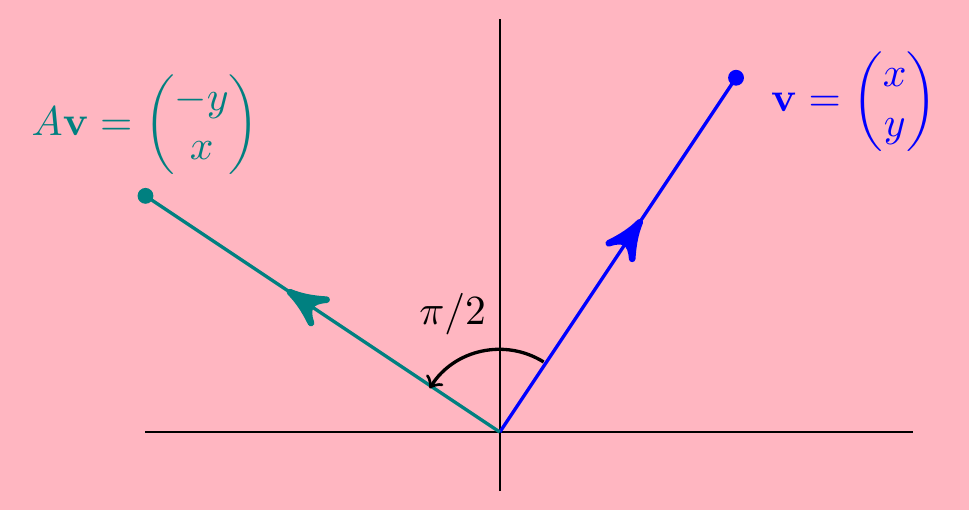
Consider the matrix $A=\begin{pmatrix} 0 & -1 \\ 1 & 0 \end{pmatrix}$ mapping $\;\;\begin{pmatrix} x \\ y \end{pmatrix}\longmapsto \begin{pmatrix} 0 & -1 \\ 1 & 0 \end{pmatrix} \begin{pmatrix} x \\ y \end{pmatrix} =\begin{pmatrix} -y \\ x \end{pmatrix}$.

This rotates vectors anti-clockwise around the origin by a right angle $\pi/2$.

Now we said that a transformation ${\bf v}\mapsto A{\bf v}$ doesn’t alter the direction of its eigenvectors. But surely a rotation angle $\pi/2$ about the origin will change the direction of every non-zero vector - it seems we have a matrix with no eigenvalues or eigenvectors? The answer is that eigenvalues (and eigenvectors) can be complex.

Indeed, the characteristic polynomial of $A$ is \[\begin{align*} \det(A-\lambda I) =\begin{vmatrix} -\lambda & -1 \\ 1 & -\lambda \end{vmatrix} =\lambda^2+1 \end{align*}\] and so the eigenvalues are $\lambda=\pm i$.

To find the corresponding eigenspace for $\lambda=i$, we find ${\bf v}=\begin{pmatrix} x \\ y \end{pmatrix}$ such that $(A-iI){\bf v}={\bf 0}$

\[\left(\!\!\begin{array}{cc|c} -i & -1 & 0 \\ 1 & -i & 0 \end{array}\!\!\right) \xrightarrow{iR_1} \left(\!\!\begin{array}{cc|c} 1 & -i & 0 \\ 1 & -i & 0 \end{array}\!\!\right) \xrightarrow{R_2-R_1} \left(\!\!\begin{array}{cc|c} 1 & -i & 0 \\ 0 & 0 & 0 \end{array}\!\!\right).\]

This means $x=iy$ and the corresponding eigenspace is $V_{i}=\operatorname{Span}\left\{\begin{pmatrix} i \\ 1 \end{pmatrix}\right\}$.

Similarly, we can show that the eigenspace corresponding to $\lambda=-i$ is $\;V_{-i}=\operatorname{Span}\left\{\begin{pmatrix} 1 \\ i \end{pmatrix}\right\}$.

The rotation doesn’t change the “directions” of these complex vectors!

3.12 Diagonalisation

One important application of eigenvalues and eigenvectors is to diagonalise a matrix $A$, which means finding a matrix $Y$ such that \[ Y^{-1}AY = D \] where $D$ is a diagonal matrix. As we saw in the Linear Algebra topic, diagonal matrices are much easier to handle.

The trick to finding such a matrix $Y$ is to choose its columns to be linearly independent eigenvectors of $A$.

Example. $\,$ Find a matrix $Y$ that diagonalises the matrix $A=\begin{pmatrix} 2 & 2 \\ 0 & 4 \end{pmatrix}$.

In the last section we found the eigenvalues $\lambda_1=2$, $\lambda_2=4$, with corresponding independent eigenvectors ${\bf v}_1=\begin{pmatrix} 1 \\ 0 \end{pmatrix}$ and ${\bf v}_2=\begin{pmatrix} 1 \\ 1 \end{pmatrix}$. So let’s try $Y=\big( {\bf v}_1 \big| {\bf v}_2 \big) = \begin{pmatrix} 1 & 1 \\ 0 & 1 \end{pmatrix}$. Then \[\begin{align*} Y^{-1}AY &= \begin{pmatrix} 1 & -1 \\ 0 & 1 \end{pmatrix} \begin{pmatrix} 2 & 2 \\ 0 & 4 \end{pmatrix} \begin{pmatrix} 1 & 1 \\ 0 & 1 \end{pmatrix} \\ &= \begin{pmatrix} 1 & -1 \\ 0 & 1 \end{pmatrix} \begin{pmatrix} 2 & 4 \\ 0 & 4 \end{pmatrix} = \begin{pmatrix} 2 & 0 \\ 0 & 4 \end{pmatrix}. \end{align*}\] This matrix is indeed diagonal. Furthermore, notice that its entries are the eigenvalues $\lambda_1$ and $\lambda_2$. This is not a coincidence!

For a given $A$, the matrix $Y$ is not unique. Suppose we wrote the eigenvectors the other way around, setting $Y=\begin{pmatrix} 1 & 1 \\ 1 & 0 \end{pmatrix}$. Then \[Y^{-1}AY = \begin{pmatrix} 0 & 1 \\ 1 & -1 \end{pmatrix} \begin{pmatrix} 2 & 2 \\ 0 & 4 \end{pmatrix} \begin{pmatrix} 1 & 1 \\ 1 & 0 \end{pmatrix} = \begin{pmatrix} 4 & 0 \\ 0 & 2 \end{pmatrix}, \] so the order of the eigenvectors in $D$ is swapped, but we still diagonalised $A$ and this time the eigenvalues swapped in $D$ as well.

Alternatively, if we chose instead the eigenvector ${\bf v}_2=\begin{pmatrix} -2 \\ -2 \end{pmatrix}$, so that $Y=\begin{pmatrix} 1 & -2 \\ 0 & -2 \end{pmatrix}$, then \[\begin{align*} Y^{-1}AY &= \begin{pmatrix} 1 & -1 \\ 0 & -\frac12 \end{pmatrix} \begin{pmatrix} 2 & 2 \\ 0 & 4 \end{pmatrix} \begin{pmatrix} 1 & -2 \\ 0 & -2 \end{pmatrix} \\ &= \begin{pmatrix} 2 & 0 \\ 0 & 4 \end{pmatrix}. \end{align*}\] So it doesn’t seem to matter which eigenvectors we choose, except for the order we write them.

To explain why this works, suppose $A$ is an $n\times n$ matrix with (not necessarily distinct) eigenvalues $\lambda_1,...,\lambda_n$ and corresponding eigenvectors ${\bf v}_1,...,{\bf v}_n$ so that $A{\bf v}_i=\lambda_i{\bf v}_i$.

\[Y=\Biggl({\bf v}_1 \; \Big|\; {\bf v}_2 \; \Big| \; ... \; \Big| \; {\bf v}_n \Biggr) \qquad\text{and}\qquad D=\begin{pmatrix} \lambda_1 & 0 & \cdots & 0 \\ 0 & \lambda_2 & \cdots & 0 \\ \vdots & \vdots & \ddots & \vdots \\ 0 & 0 & \cdots & \lambda_n \end{pmatrix}.\]

Due to the way matrix multiplication is defined, the columns of $AY$ are precisely $A$ times the columns of $Y$, i.e. they are $A{\bf v}_i=\lambda_i{\bf v}_i$: \[\begin{align*} AY=A\Biggl({\bf v}_1 \; \Big|\; {\bf v}_2 \; \Big| \; ... \; \Big| \; {\bf v}_n \Biggr) &=\Biggl(A{\bf v}_1 \; \Big|\; A{\bf v}_2 \; \Big| \; ... \; \Big| \; A{\bf v}_n \Biggr) \\ &=\Biggl(\lambda_1{\bf v}_1 \; \Big|\; \lambda_2{\bf v}_2 \; \Big| \; ... \; \Big| \; \lambda_n{\bf v}_n \Biggr). \end{align*}\] On the other hand, the columns of $YD$ are the columns of $Y$ multiplied by the corresponding diagonal entries of $D$: \[\begin{align*} YD &= \Biggl({\bf v}_1 \; \Big|\; {\bf v}_2 \; \Big| \; ... \; \Big| \; {\bf v}_n \Biggr) \begin{pmatrix} \lambda_1 & 0 & \cdots & 0 \\ 0 & \lambda_2 & \cdots & 0 \\ \vdots & \vdots & \ddots & \vdots \\ 0 & 0 & \cdots & \lambda_n \end{pmatrix} \\ &=\Biggl(\lambda_1{\bf v}_1 \; \Big|\; \lambda_2{\bf v}_2 \; \Big| \; ... \; \Big| \; \lambda_n{\bf v}_n \Biggr). \end{align*}\] In particular, we see that $AY=YD$. Now provided that $Y$ is invertible, we get the diagonalisation $A=Y^{-1}AY$. But we need $Y^{-1}$ to exist for this to work. This will happen if the vectors $\{{\bf v}_1,...,{\bf v}_n\}$ are a basis for $\mathbb{R}^n$, since then the determinant $\det(Y)\neq 0$ and $Y$ is invertible.

Example. $\,$ Now consider the matrix $A = \begin{pmatrix} 3 & 1 \\ 0 & 3 \end{pmatrix}$. In the last section, we saw it has a repeated eigenvalue $\lambda=3.$ The eigenspace $V_3 = \operatorname{Span}\left\{\begin{pmatrix} 1 \\ 0 \end{pmatrix}\right\}$ is only one-dimensional and we can only choose one linearly independent eigenvector, e.g. ${\bf v}=\begin{pmatrix} 1 \\ 0 \end{pmatrix}$.

We don’t have enough independent eigenvectors to put in the matrix $Y$ to make it invertible so the above method of diagonalisation will not work.

In fact no $Y$ exists such that $Y^{-1}AY$ is diagonal. If $Y=\begin{pmatrix} a & b \\ c & d \end{pmatrix}$ and $D=\begin{pmatrix} r & 0 \\ 0 & s \end{pmatrix}$ then \[\begin{align*} AY=YD &\quad\implies\quad \begin{pmatrix} 3 & 1 \\ 0 & 3 \end{pmatrix} \begin{pmatrix} a & b \\ c & d \end{pmatrix} =\begin{pmatrix} a & b \\ c & d \end{pmatrix} \begin{pmatrix} r & 0 \\ 0 & s \end{pmatrix} \\ &\quad\implies\quad \begin{cases} \,3a+c=ar, & \,3b+d=bs \\ \quad\;\;\; 3c=cr, & \quad\;\;\; 3d=ds \end{cases} \end{align*}\] Assuming $c\neq 0$ we get $r=3 \implies 3a+c=ra=3a\implies c=0$, a contradiction, so we must have $c=0$. Similarly, $d=0$ but then the matrix $P$ isn’t invertible as it has a row of zeros.

One can more rigorously show that a square matrix $A$ is diagonalisable if and only if there is a basis consisting of eigenvectors. Notice it is the number of independent eigenvectors that matters, not the number of distinct eigenvalues. A matrix can have repeated eigenvalues and still be diagonalisable.
It can also be proved that symmetric $n\times n$ matrices (with real coefficients) always have a basis of $n$ eigenvectors, and hence are always diagonalisable.
In fact, if a matrix is not diagonalisable, there is something called the Jordan normal form which “almost” diagonalises the matrix.

Eigenvectors corresponding to different eigenvalues are automatically linearly independent. A sketch of why this is true is as follows. Suppose $A{\bf v}_1=\lambda_1{\bf v}_1$ and $A{\bf v}_2=\lambda_2{\bf v}_2$ for the same matrix $A$, with $\lambda_1\neq \lambda_2$. Then \[\begin{align*} a{\bf v}_1 + b{\bf v}_2 = \boldsymbol{0} &\quad\implies\quad (A-\lambda_1I)(a{\bf v}_1 + b{\bf v}_2) = \boldsymbol{0}\\ &\quad\implies\quad (A-\lambda_1I)b{\bf v}_2 = \boldsymbol{0}\\ &\quad\implies\quad (\lambda_2-\lambda_1)b{\bf v}_2 = \boldsymbol{0} \end{align*}\] Since $\lambda_1\neq\lambda_2$ and ${\bf v}_2\neq \boldsymbol{0}$ by definition, this is only possible if $b=0$. But then $a{\bf v}_1=\boldsymbol{0}$, and since ${\bf v}_1\neq \boldsymbol{0}$ we see that $a=0$. There is therefore no linear combination of ${\bf v}_1$ and ${\bf v}_2$ that gives $\boldsymbol{0}$, so they are linearly independent.

Example. $\,$ Find a matrix $Y$ that diagonalises the matrix $A=\begin{pmatrix}5 & 6 & -3\\ 0 & -1 & 0\\ 6 & 6 & -4 \end{pmatrix}$.

Previously we found:

an eigenvalue $\lambda=2$ with eigenspace $\operatorname{Span}\left\{\begin{pmatrix} 1 \\ 0 \\ 1 \end{pmatrix}\right\}$.
a repeated eigenvalue $\lambda=-1$ with eigenspace $\operatorname{Span}\left\{\begin{pmatrix} 1 \\ 0 \\ 2 \end{pmatrix}, \begin{pmatrix} 0 \\ 1 \\ 2 \end{pmatrix}\right\}$

So if we take $Y = \begin{pmatrix} 1 & 1 & 0 \\ 0 & 0 & 1 \\ 1 & 2 & 2 \end{pmatrix},$ then $D=Y^{-1}AY = \begin{pmatrix} 2 & 0 & 0 \\ 0 & -1 & 0 \\ 0 & 0 & -1 \end{pmatrix}.$

It’s a good idea to check that this really works. Multiply out the matrices $AY=YD$ and check you didn’t go wrong during the calculation.

Diagonalisation has important applications in physics, chemistry, mechanics,… as well as in simultaneous differential equations, which we will see next term. Here we will finish with a couple of simple applications involving powers of matrices.

Example. $\,$ Given $A=\begin{pmatrix} 2 & 2 \\ 0 & 4 \end{pmatrix}$, calculate $A^{100}$.

Using $A=YDY^{-1}$, with the $Y=\begin{pmatrix} 1 & 1 \\ 0 & 1 \end{pmatrix}$ and $D=\begin{pmatrix} 2 & 0 \\ 0 & 4 \end{pmatrix}$ we found before, we have \[\begin{align*} A^{100} = (YDY^{-1})^{100} &= YDY^{-1}YDY^{-1}\ldots YDY^{-1}YDY^{-1} \\ &= YD^{100}Y^{-1}. \end{align*}\] But finding $D^{100}$ is easy – just raise the diagonal elements to the power $100$. So \[\begin{align*} A^{100} &= \begin{pmatrix} 1 & 1 \\ 0 & 1 \end{pmatrix} \begin{pmatrix} 2^{100} & 0 \\ 0 & 4^{100} \end{pmatrix} \begin{pmatrix} 1 & -1 \\ 0 & 1 \end{pmatrix} \\ &= \begin{pmatrix} 2^{100} & 4^{100}-2^{100} \\ 0 & 4^{100} \end{pmatrix}. \end{align*}\]

The same kind of trick works for finding “roots” of matrices. The point is finding a root of a diagonal matrix is easier, so the diagonalisation process allows us to shift the problem to these instead.

Example. $\,$ Find a matrix $B$ such that $B^3=A=\begin{pmatrix} -46 & 135 \\ -18 & 53 \end{pmatrix}$.

We first find the eigenvalues: \[\begin{align*} \det(A-\lambda I) &= \begin{vmatrix} -46-\lambda & 135 \\ -18 & 53-\lambda \end{vmatrix} \\ &=\lambda^2-7\lambda-8=(\lambda+1)(\lambda-8) \end{align*}\] so the eigenvalues are $\lambda_1=-1$ and $\lambda_2=8$.

For $\lambda_1=-1$, we solve $(A+I){\bf v}_1={\bf 0}$, i.e. \[ \left(\begin{matrix} -45 & 135 \\ -18 & 54 \end{matrix} \left|\,\begin{matrix} 0 \\ 0 \end{matrix}\right.\right) \longrightarrow \left(\begin{matrix} 1 & -3 \\ 0 & 0 \end{matrix} \left|\,\begin{matrix} 0 \\ 0 \end{matrix}\right.\right). \] Hence we can take ${\bf v}_1=\begin{pmatrix} 3 \\ 1 \end{pmatrix}$ as the corresponding eigenvector.

For $\lambda_1=8$, we solve $(A-8I){\bf v}_2={\bf 0}$, i.e. \[ \left(\begin{matrix} -54 & 135 \\ -18 & 45 \end{matrix} \left|\,\begin{matrix} 0 \\ 0 \end{matrix}\right.\right) \longrightarrow \left(\begin{matrix} 2 & -5 \\ 0 & 0 \end{matrix} \left|\,\begin{matrix} 0 \\ 0 \end{matrix}\right.\right). \] Hence we can take ${\bf v}_2=\begin{pmatrix} 5 \\ 2 \end{pmatrix}$ as the corresponding eigenvector.

We now have $Y^{-1}AY=D$ where $Y=\begin{pmatrix} 3 & 5 \\ 1 & 2 \end{pmatrix}$ and $D=\begin{pmatrix} -1 & 0 \\ 0 & 8 \end{pmatrix}$. (Check this!)

Writing down a cube root of a diagonal matrix is easy - just take cube roots of the diagonal elements. In other words, $C^3=D$ where $C=\begin{pmatrix} -1 & 0 \\ 0 & 2 \end{pmatrix}$. But then letting $B=YCY^{-1}$ gives \[B^3=\left(YCY^{-1}\right)^3=YC^3Y^{-1}=YDY^{-1}=A\] and this matrix $B$ is what we are looking for:

\[\begin{align*} B=YCY^{-1} &= \begin{pmatrix} 3 & 5 \\ 1 & 2 \end{pmatrix} \begin{pmatrix} -1 & 0 \\ 0 & 2 \end{pmatrix} \begin{pmatrix} 2 & -5 \\ -1 & 3 \end{pmatrix} \\ &= \begin{pmatrix} -16 & 45 \\ -6 & 17 \end{pmatrix}. \end{align*}\]