Maths for Engineers & Scientists (MATH1551)
Topic 1 - Linear Algebra
1.0 Introduction
In engineering and science, we often need to solve simultaneous equations like \[\begin{align*} 20x \qquad\;\;\, - 15z &= 220, \\ 25y - 10z &= 0, \\ -15x - 10y + 45z &= 0. \end{align*}\] This a system of linear equations, where “linear” means they only involve first powers of the variables (so constant multiples of \(x\), \(y\) and \(z\) but nothing like \(x^2\) or \(\sin{z}\)). By “solve”, we mean find values for \(x\), \(y\) and \(z\) that satisfy all the equations simultaneously. Linear Algebra begins with the study of systems like this. Here is an example of a problem that would give rise to the equations above.
Example. \(\,\) Currents in an electrical network leading to linear equations.
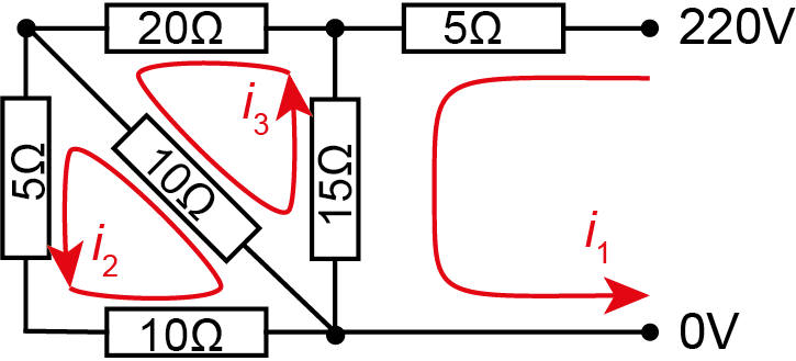
Kirchoff’s law tells us that the sum of voltage drops is equal to the sum of voltage sources around any loop. Applying it to the three loops shown, along with Ohm’s law for each resistor, gives the simultaneous equations \[\begin{align*} 5i_1 + 15(i_1 - i_3) &= 220, \\ 10(i_2 - i_3) + 5i_2 + 10i_2 &= 0, \\ 20i_3 + 10(i_3-i_2) + 15(i_3-i_1) &= 0. \end{align*}\] Simplifying, we get our original system \[\begin{align*} 20i_1 \qquad\;\;\,- 15i_3 &= 220, \\ 25i_2 - 10i_3 &= 0, \\ -15i_1 - 10i_2 + 45i_3 &= 0. \end{align*}\]
An electrical engineer faced with these equations might use MATLAB and type
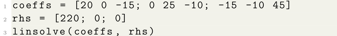
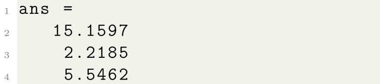
This will output the solutions for \(x\), \(y\), \(z\), or equivalently the currents \(i_1\), \(i_2\) and \(i_3\):
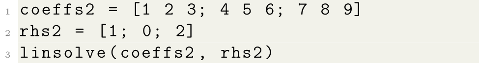
In this topic, we’ll learn how the computer found this solution (a method called Gaussian elimination). It’s important to understand the basics of what is happening “under the hood” because it doesn’t always work as smoothly as this. Consider the equations \[\begin{align*} x + 2y + 3z &= 1, \\ 4x + 5y + 6z &= 0, \\ 7x + 8y + 9z &= 2. \end{align*}\] If we try to solve this system in MATLAB as before, typing
we get the output
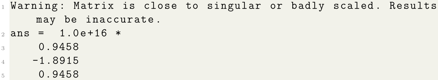
The warning message gives us a clue that something is amiss. In fact, not only does this “solution” not satisfy the original equations, actually no solution exists! This issue has come about purely due to rounding error in the computer. We’ll see how to determine whether a system of equations has a solution or not, using the determinant.
Another thing that can go wrong is that the calculation with Gaussian elimination is too slow, particularly for large systems of equations. Although we will concentrate on small systems (for practical reasons!), we’ll also learn about some alternative iterative methods that come into their own for the large linear systems often encountered in science and engineering. Large systems of equations often arise from spatial problems such as the following.
Example. \(\,\) In studying a steady state temperature in a square with top and left sides held at \(100^\circ\)C and bottom and right at \(0^\circ\)C, a typical numerical approach is to divide into a discrete grid of points. For example, taking \(N=16\) points \(x_1,\ldots, x_{16}\):
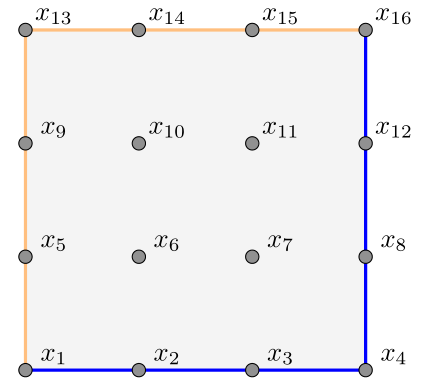
In a steady state, the temperature at an interior point is (approximately) the average of its four neighbours. The values on the edges are fixed at \[\begin{align*} &x_1=x_{5}=x_9=x_{13}=x_{14}=x_{15}=x_{16}=100, \\ &x_2=x_3=x_4=x_8=x_{12} = 0, \end{align*}\] leaving only four unknowns remaining for the interior values, determined by \[\begin{align*} -\tfrac14x_2 - \tfrac14x_5 + x_6 - \tfrac14x_7 - \tfrac14x_{10} &= 0, \\ -\tfrac14x_3 - \tfrac14x_6 + x_7 - \tfrac14x_8 - \tfrac14x_{11} &= 0, \\ -\tfrac14x_6 - \tfrac14x_9 + x_{10} - \tfrac14x_{11} - \tfrac14x_{14} &= 0, \\ -\tfrac14x_7 - \tfrac14x_{10} + x_{11} - \tfrac14x_{12} - \tfrac14x_{15} &= 0. \end{align*}\]
Increasing the resolution quickly increases the number of equations. For instance, with \(N=32^2\) and \(N=128^2\), MATLAB produces
\(\hskip1cm\)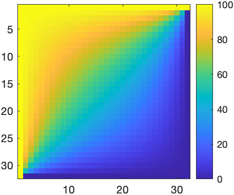 \(\hskip1cm\)
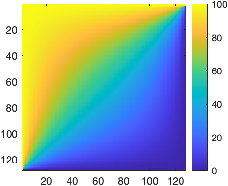
Increasing the resolution even further requires alternative “cleverer” methods, and maybe you can see how further problems arise in three-dimensional calculations.
Let’s finish by thinking about what would make a system of three equations easier to solve. The easiest case would be a diagonal system where the equations are decoupled, for example \[\begin{align*} x \qquad\qquad &= 2, \\ -y\qquad &= 1, \\ 2z &= 6. \end{align*}\] We can just read off the solution here, giving \(x=2\), \(y=-1\), \(z=3\).
The next simplest system is one that is triangular in form, for example \[\begin{align*} x + 2y -\;\; z &= -3, \\ y - 3z &= -10, \\ z &= \;\;\,3. \end{align*}\] We can solve this system by back substitution: first find \(z=3\) from the last equation. Then substitute this into the second equation to find \(y-9=-10\), giving \(y=-1\). Finally substitute these values of \(y\) and \(z\) into the first equation to find \(x-5 = -3\), giving \(x=2\).
1.1 Gaussian elimination
The idea behind Gaussian elimination is to systematically convert a linear system into a more convenient form that can be solved easily.
Sometimes textbooks convert to triangular form, which can then be solved quickly by back substitution. Other times, they like to go further and transform the system to a completely decoupled diagonal form where you can just read off the answer. This second way is useful but can take longer (more steps) and often, numerical software (like Matlab or numpy/python) do the first “triangular” way.
So how do we “transform” the system from one form to another? There are three simple operations we can perform that don’t change the solution:
\(\quad\left(R_i\leftrightarrow R_j\right):\;\)
Swap two equations.
For example,
\[
\begin{split}
x + 2y - \;\,z &= -3\\
x + \;\,y + 2z &= \;\;\,7\\
2x + 5y - 4z &= -13
\end{split}
\quad \xrightarrow{R_1\leftrightarrow R_2}
\quad
\begin{split}
x + \;\,y + 2z &= \;\;\,7\\
x + 2y - \;\,z &= -3\\
2x + 5y - 4z &= -13
\end{split}
\]
\(\quad\left(cR_i\right):\;\)
Multiply an equation by a non-zero constant.
For example,
\[
\begin{split}
x + 2y - \;\,z &= -3\\
x + \;\,y + 2z &= \;\;\,7\\
2x + 5y - 4z &= -13
\end{split}
\quad \xrightarrow{3R_1}
\quad
\begin{split}
3x + 6y - 3z &= -9\\
x + \;\,y + 2z &= \;\;\,7\\
2x + 5y - 4z &= -13
\end{split}
\]
\(\quad\left(R_i+cR_j\right):\;\)
Add/subtract a multiple of one equation to another.
For example,
\[
\begin{split}
x + 2y - \;\,z &= -3\\
x + \;\,y + 2z &= \;\;\,7\\
2x + 5y - 4z &= -13
\end{split}
\quad \xrightarrow{R_3 - 2R_1}
\quad
\begin{split}
x + 2y - \;\,z &= -3\\
x + \;\,y + 2z &= \;\;\,7\\
y - 2z &= -7
\end{split}
\]
Hopefully you can see these operations don’t affect the solutions to the system. They are called elementary row operations (EROs). When performing these operations, it is useful to have concise notation for the system. We simply drop the unnecessary symbols, just keeping the numbers written in a so-called augmented matrix. For example, \[ \begin{split} x + 2y - \;\,z &= -3\\ x + \;\,y + 2z &= \;\;\,7\\ 2x + 5y - 4z &= -13 \end{split} \qquad\text{becomes}\qquad \left(\begin{matrix} 1 & 2 & -1 \\ 1 & 1 & 2 \\ 2 & 5 & -4 \end{matrix} \left|\,\begin{matrix} -3 \\ 7 \\ -13 \end{matrix}\right.\right) \] Notice that the right-hand sides (the constant terms) of the equations are to the right of the vertical line. So our aim in Gaussian elimination is to transform this into the triangular form looking like \[\left(\begin{matrix} 1 & ? & ? \\ 0 & 1 & ? \\ 0 & 0 & 1 \end{matrix} \left|\,\begin{matrix} ? \\ ? \\ ? \end{matrix}\right.\right). \] There is a systematic algorithm, which is easiest to illustrate with examples.
Example. \(\,\) Gaussian elimination for the above \(3\times3\) system. We want to obtain zeros below the diagonal and it’s convenient to do this one column at a time, starting from the left. First, eliminate \(x\) from \(R_2\) and \(R_3\) by subtracting appropriate multiples of \(R_1\): \[ \left(\begin{matrix} 1 & 2 & -1 \\ 1 & 1 & 2 \\ 2 & 5 & -4 \end{matrix} \left|\,\begin{matrix} -3 \\ 7 \\ -13 \end{matrix}\right.\right) \xrightarrow{R_2 - R_1} \left(\begin{matrix} 1 & 2 & -1 \\ 0 & -1 & 3 \\ 2 & 5 & -4 \end{matrix} \left|\,\begin{matrix} -3 \\ 10 \\ -13 \end{matrix}\right.\right)\] \[\hspace{4.5cm} \xrightarrow{R_3 - 2R_1} \left(\begin{matrix} 1 & 2 & -1 \\ 0 & -1 & 3 \\ 0 & 1 & -2 \end{matrix} \left|\,\begin{matrix} -3 \\ 10 \\ -7 \end{matrix}\right.\right) \] Next we change the coefficient of \(y\) in \(R_2\) to 1, by multiplying \(R_2\) by \(-1\): \[ \left(\begin{matrix} 1 & 2 & -1 \\ 0 & -1 & 3 \\ 0 & 1 & -2 \end{matrix} \left|\,\begin{matrix} -3 \\ 10 \\ -7 \end{matrix}\right.\right) \xrightarrow{-R_2} \left(\begin{matrix} 1 & 2 & -1 \\ 0 & 1 & -3 \\ 0 & 1 & -2 \end{matrix} \left|\,\begin{matrix} -3 \\ -10 \\ -7 \end{matrix}\right.\right)\] Finally, we eliminate \(y\) from \(R_3\) by subtracting an appropriate multiple of \(R_2\): \[ \left(\begin{matrix} 1 & 2 & -1 \\ 0 & 1 & -3 \\ 0 & 1 & -2 \end{matrix} \left|\,\begin{matrix} -3 \\ -10 \\ -7 \end{matrix}\right.\right) \xrightarrow{R_3-R_2} \left(\begin{matrix} 1 & 2 & -1 \\ 0 & 1 & -3 \\ 0 & 0 & 1 \end{matrix} \left|\,\begin{matrix} -3 \\ -10 \\ 3 \end{matrix}\right.\right) \] We have reached the triangular form that we hoped for, with 1’s on the diagonal, and we could go on to solve by back substitution.
Depending on the initial system, it could be that we need to swap rows somewhere.
Example. \(\,\) Use Gaussian elimination to transform the system \[\left(\begin{matrix} 0 & 0 & 3 \\ 1 & 2 & 1 \\ 2 & 1 & 0 \end{matrix} \left|\,\begin{matrix} 9 \\ 0 \\ 3 \end{matrix}\right.\right) \] to triangular form, and hence find the solution by back substitution. The top-left element is zero, so we can’t eliminate \(x\) from \(R_2\) and \(R_3\) by subtracting multiples of \(R_1\). Instead, we swap \(R_1\) and \(R_2\) first: \[ \left(\begin{matrix} 0 & 0 & 3 \\ 1 & 2 & 1 \\ 2 & 1 & 0 \end{matrix} \left|\,\begin{matrix} 9 \\ 0 \\ 3 \end{matrix}\right.\right) \xrightarrow{R_1\leftrightarrow R_2} \left(\begin{matrix} 1 & 2 & 1 \\ 0 & 0 & 3 \\ 2 & 1 & 0 \end{matrix} \left|\,\begin{matrix} 0 \\ 9 \\ 3 \end{matrix}\right.\right) \] \[\hspace{4.5cm} \xrightarrow{R_3 - 2R_1} \left(\begin{matrix} 1 & 2 & 1 \\ 0 & 0 & 3 \\ 0 & -3 & -2 \end{matrix} \left|\,\begin{matrix} 0 \\ 9 \\ 3 \end{matrix}\right.\right) \] Now we have the same problem again: we can’t eliminate \(y\) from \(R_3\) by subtracting a multiple of \(R_2\). So we swap \(R_2\) and \(R_3\). \[ \left(\begin{matrix} 1 & 2 & 1 \\ 0 & 0 & 3 \\ 0 & -3 & -2 \end{matrix} \left|\,\begin{matrix} 0 \\ 9 \\ 3 \end{matrix}\right.\right) \xrightarrow{R_2\leftrightarrow R_3} \left(\begin{matrix} 1 & 2 & 1 \\ 0 & -3 & -2 \\ 0 & 0 & 3 \end{matrix} \left|\,\begin{matrix} 0 \\ 3 \\ 9 \end{matrix}\right.\right) \] Now we can reach triangular form just by scaling \(R_2\) and \(R_3\): \[ \left(\begin{matrix} 1 & 2 & 1 \\ 0 & -3 & -2 \\ 0 & 0 & 3 \end{matrix} \left|\,\begin{matrix} 0 \\ 3 \\ 9 \end{matrix}\right.\right) \xrightarrow{-\tfrac13R_2} \left(\begin{matrix} 1 & 2 & 1 \\ 0 & 1 & \tfrac23 \\ 0 & 0 & 3 \end{matrix} \left|\,\begin{matrix} 0 \\[2pt] -1 \\[2pt] 9 \end{matrix}\right.\right) \] \[\hspace{4.5cm} \xrightarrow{\tfrac13R_3} \left(\begin{matrix} 1 & 2 & 1 \\ 0 & 1 & \tfrac23 \\ 0 & 0 & 1 \end{matrix} \left|\,\begin{matrix} 0 \\[2pt] -1 \\[2pt] 3 \end{matrix}\right.\right) \] Back substitution then gives the solution \[\begin{align*} z &= 3, \\ y &= -1-\tfrac23z = -1-\tfrac23(3) = -3, \\ x &= 0-2y-z = 0-2(-3)-3 = 3. \end{align*}\]
To finish, let’s show how transforming a system into a diagonal form works.
Example. \(\,\) Gaussian elimination for the previous example to diagonal form. Once we’ve reached the triangular form as above, we just have to obtain zeros above the diagonal as well as below. This time we start with the last column, subtracting appropriate multiples of the bottom row: \[ \left(\begin{matrix} 1 & 2 & 1 \\ 0 & 1 & \tfrac23 \\ 0 & 0 & 1 \end{matrix} \left|\,\begin{matrix} 0 \\[2pt] -1 \\[2pt] 3 \end{matrix}\right.\right) \xrightarrow{R_2-\tfrac23R_3} \left(\begin{matrix} 1 & 2 & 1 \\ 0 & 1 & 0 \\ 0 & 0 & 1 \end{matrix} \left|\,\begin{matrix} 0 \\ -3 \\ 3 \end{matrix}\right.\right) \] \[\hspace{4.5cm} \xrightarrow{R_1 - R_3} \left(\begin{matrix} 1 & 2 & 0 \\ 0 & 1 & 0 \\ 0 & 0 & 1 \end{matrix} \left|\,\begin{matrix} -3 \\ -3 \\ 3 \end{matrix}\right.\right) \] and then eliminate the \(y\) from \(R_1\) using the middle row: \[ \left(\begin{matrix} 1 & 2 & 0 \\ 0 & 1 & 0 \\ 0 & 0 & 1 \end{matrix} \left|\,\begin{matrix} -3 \\ -3 \\ 3 \end{matrix}\right.\right) \xrightarrow{R_1-2R_2} \left(\begin{matrix} 1 & 0 & 0 \\ 0 & 1 & 0 \\ 0 & 0 & 1 \end{matrix} \left|\,\begin{matrix} 3 \\ -3 \\ 3 \end{matrix}\right.\right) \] We can now read off the solution as the three equations simply say \[\begin{align*} x \qquad\qquad &= \;\,3, \\ y \qquad &= -3, \\ z &= \;\,3. \end{align*}\]
It’s very important to apply EROs to the whole rows of an augmented matrix, not just the left hand side. If you forget about the part on the right side of the vertical bar, it won’t work!
In the above examples, we deliberately wrote the specific EROs as part of the calculations. You should always do this as well in assignments and the exam. It tells the reader what you’re doing and also helps you in case there’s a mistake and you need to go back and fix things.
It’s possible to perform more than one operation at once. However, you should be careful doing this and, if in doubt, do one ERO at each step. In particular, never apply two operations to the same row in the same step.
Swapping rows to get non-zero elements in the right position is called pivoting, and these key entries (that have to be non-zero) are called pivots. We’ll see more about this later.
\(\,\)
There are some things that can go wrong with the above method, however, because…
\(\,\)
1.2 Solvability
…not all systems of linear equations have a solution and sometimes they have lots. We can see this happening even in a \(2\times 2\) system. For example, consider the equations \[\begin{align*} mx - y &= -c, \\ y &= 0, \end{align*}\] where \(m\) and \(c\) are constants. Graphically, these equations correspond to two straight lines, and provided that \(m\neq 0\), there is a unique solution at the point of intersection \(x=-c/m\), \(y=0\):
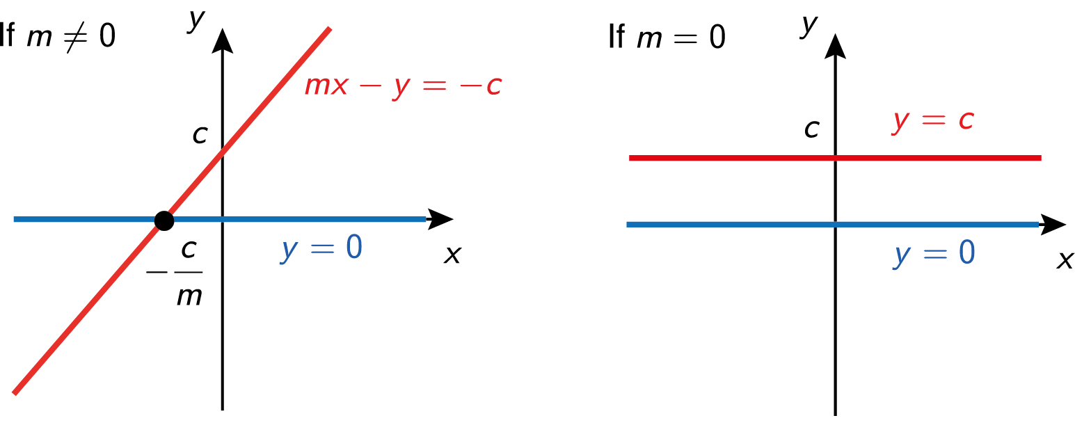
On the other hand, when \(m=0\), the lines are parallel and two things can happen, depending on \(c\).
If \(c\neq 0\), the lines are distinct, the equations are inconsistent, and there are no solutions.
If \(c=0\), the two lines are the same, the two equations are insufficient
to determine both \(x\) and \(y\) uniquely, and there are infinitely many solutions.
This behaviour is typical of linear systems of any size: for “most” values of the coefficients, there is a unique solution for any right-hand side values. But for certain values of the coefficients, there can be either no solutions or an infinite number, depending on the right-hand side. Let’s see how these pathological situations manifest themselves when we try to do Gaussian elimination on some \(3\times3\) systems.
Example. \(\,\) Apply Gaussian elimination to the system \[\begin{align*} x + 2y + 3z &= \;\,1, \\ 4x + 5y + 6z &= \;\,1, \\ 7x + 8y + 9z &= -5. \end{align*}\] We write the system in augmented matrix form and proceed as before: \[ \left(\begin{matrix} 1 & 2 & 3 \\ 4 & 5 & 6 \\ 7 & 8 & 9 \end{matrix} \left|\,\begin{matrix} 1 \\ 1 \\ -5 \end{matrix}\right.\right) \xrightarrow{R_2-4R_1} \left(\begin{matrix} 1 & 2 & 3 \\ 0 & -3 & -6 \\ 7 & 8 & 9 \end{matrix} \left|\,\begin{matrix} 1 \\ -3 \\ -5 \end{matrix}\right.\right) \] \[\xrightarrow{R_3-7R_3} \left(\begin{matrix} 1 & 2 & 3 \\ 0 & -3 & -6 \\ 0 & -6 & -12 \end{matrix} \left|\,\begin{matrix} 1 \\ -3 \\ -12 \end{matrix}\right.\right) \xrightarrow{-\tfrac13R_2} \left(\begin{matrix} 1 & 2 & 3 \\ 0 & 1 & 2 \\ 0 & -6 & -12 \end{matrix} \left|\,\begin{matrix} 1 \\ 1 \\ -12 \end{matrix}\right.\right)\] \[\hspace{5.7cm} \xrightarrow{R_3+6R_2} \left(\begin{matrix} 1 & 2 & 3 \\ 0 & 1 & 2 \\ 0 & 0 & 0 \end{matrix} \left|\,\begin{matrix} 1 \\ 1 \\ -6 \end{matrix}\right.\right). \] The last equation says that \(0=-6\), which is false! This means the system of equations is inconsistent: there are no solutions (like with the distinct parallel lines).
Example. \(\,\) Apply Gaussian elimination to the system \[\begin{align*} x + 2y + 3z &= 1, \\ 4x + 5y + 6z &= 1, \\ 7x + 8y + 9z &= 1. \end{align*}\] This is the same as the last example but with different right-hand side in the last equation. Gaussian elimination will involve the same sequence of row operations, since these don’t depend on the right-hand side (think about why). Thus we get \[ \left(\begin{matrix} 1 & 2 & 3 \\ 4 & 5 & 6 \\ 7 & 8 & 9 \end{matrix} \left|\,\begin{matrix} 1 \\ 1 \\ 1 \end{matrix}\right.\right) \xrightarrow{R_2-4R_1} \left(\begin{matrix} 1 & 2 & 3 \\ 0 & -3 & -6 \\ 7 & 8 & 9 \end{matrix} \left|\,\begin{matrix} 1 \\ -3 \\ 1 \end{matrix}\right.\right) \] \[\hspace{0.5cm} \xrightarrow{R_3-7R_3} \left(\begin{matrix} 1 & 2 & 3 \\ 0 & -3 & -6 \\ 0 & -6 & -12 \end{matrix} \left|\,\begin{matrix} 1 \\ -3 \\ -6 \end{matrix}\right.\right) \xrightarrow{-\tfrac13R_2} \left(\begin{matrix} 1 & 2 & 3 \\ 0 & 1 & 2 \\ 0 & -6 & -12 \end{matrix} \left|\,\begin{matrix} 1 \\ 1 \\ -6 \end{matrix}\right.\right) \] \[\hspace{5.7cm} \xrightarrow{R_3+6R_2} \left(\begin{matrix} 1 & 2 & 3 \\ 0 & 1 & 2 \\ 0 & 0 & 0 \end{matrix} \left|\,\begin{matrix} 1 \\ 1 \\ 0 \end{matrix}\right.\right). \] Unlike before, the last equation is now consistent, it just says \(0=0\). But there are effectively only two equations left, \[\begin{align*} x + 2y + 3z &=1,\\ y + 2z &= 1, \end{align*}\] so only two variables can be determined, in terms of the third one (like the case where the lines were parallel and \(c=0\)). Choosing \(z\) to be the undetermined one, write \(z=\lambda\) where \(\lambda\) is an arbitrary number (called a parameter). Then back substitution gives every solution in terms of the parameter: \[\begin{align*} z &= \lambda,\\ y &= 1 - 2\lambda,\\ x &= 1 - 2(1-2\lambda) - 3\lambda = -1 + \lambda. \end{align*}\] There are infinitely many solutions, and moreover, we have found them all!
\(\,\)
We’ll see later in the course that the set of solutions to this last example is the parametric equation of a line in 3D space.
Notice that when one of the equations “drops out” like this, it is the same as starting with only two equations in the first place. Mathematicians say that the rank of the system is only 2 rather than 3.
\(\,\)
To sum up:
If you get a row of all zeros except for the right-hand side, there is no solution.
If you get a row of all zeros, and the number of non-zero rows is less than the number of variables, then the system will have multiple solutions. We can then write the answer in parametric form.
\(\,\)
1.3 Determinants
There is a way to compute ahead of time whether or not a linear system will have a unique solution.
For a \(2\times2\) system, we can derive it directly for a general system
\[\begin{align*}
ax + by &= u, \\
cx + dy &= v.
\end{align*}\]
Subtracting \(b\) times the second equation from \(d\) times the first gives
\[(ad - bc)x = du - bv.\]
Similarly, subtracting \(c\) times the first equation from \(a\) times the second gives
\[(ad - bc)y = av - cu.\]
In particular, as long as \(ad-bc\neq 0\), we find the solution is uniquely determined
\[x = \frac{du-bv}{ad-bc} \qquad\text{and}\qquad y = \frac{av - cu}{ad-bc}.\]
The denominator here is called the determinant, and is written as
\[
\begin{vmatrix}
a & b \\
c & d
\end{vmatrix} = ad-bc.
\]
So our linear system has a unique solution if the determinant is non-zero.
On the other hand, if the determinant is zero,
there will be either no solutions or infinitely many solutions
(try checking this),
just like with the \(2\times 2\) example in the previous section when \(m=0\).
Notice the determinant depends only on the coefficients \(a\), \(b\), \(c\), \(d\)
and not on \(u\), \(v\).
The situation is similar for larger systems: there is a special number called the determinant calculated from the coefficients, and the system has a unique solution if and only if its determinant is non-zero. We can evaluate the determinant by expanding along the top row. For example, \[ \begin{vmatrix} {\color{red}{a}} & {\color{red}{b}} & {\color{red}{c}} \\ d & e & f \\ g & h & i \end{vmatrix} = {\color{red}{a}}\begin{vmatrix} e & f \\ h & i \end{vmatrix} -{\color{red}{b}}\begin{vmatrix} d & f \\ g & i \end{vmatrix} +{\color{red}{c}}\begin{vmatrix} d & e \\ g & h \end{vmatrix}, \] and \[ \begin{vmatrix} {\color{red}{a}} & {\color{red}{b}} & {\color{red}{c}} & {\color{red}{d}} \\ e & f & g & h \\ i & j & k & l \\ m & n & o & p \end{vmatrix} ={\color{red}{a}}\begin{vmatrix} f & g & h \\ j & k & l \\ n & o & p \end{vmatrix} -{\color{red}{b}}\begin{vmatrix} e & g & h \\ i & k & l \\ m & o & p \end{vmatrix} \hspace{3cm}\] \[\hspace{5cm} +{\color{red}{c}}\begin{vmatrix} e & f & h \\ i & j & l \\ m & n & p \end{vmatrix} -{\color{red}{d}}\begin{vmatrix} e & f & g \\ i & j & k \\ m & n & o \end{vmatrix}. \] Hopefully you see the general pattern. Each term in the top row is multiplied by the smaller determinant obtained by crossing out the row and column of that term. Then these are added/subtracted in an alternating fashion. It’s a recursive process: a \(3\times3\) determinant is calculated using three \(2\times 2\) determinants, a \(4\times4\) determinant is calculated using four \(3\times 3\) determinants, and so on.
It’s beyond the scope of this course to derive these big formulas from scratch - the algebra gets nasty, and more complicated mathematical ideas are required. Fortunately, we just need to know how to compute them.
\(\,\)
Example. \(\,\) Calculate the determinant of the linear system \[\begin{align*} x + 2y + 3z &= 1, \\ 4x + 5y + 6z &= 1, \\ 7x + 8y + 9z &= -5. \end{align*}\] We saw earlier that this system has no solution, so it should be that the determinant vanishes. Using the \(3\times 3\) formula above, we find indeed that \[\begin{align*} \begin{vmatrix} 1 & 2 & 3\\ 4 & 5 & 6\\ 7 & 8 & 9 \end{vmatrix} &= 1\begin{vmatrix} 5 & 6\\ 8 & 9 \end{vmatrix} - 2\begin{vmatrix} 4 & 6\\ 7 & 9 \end{vmatrix} + 3\begin{vmatrix} 4 & 5\\ 7 & 8 \end{vmatrix}\\ &= 1\left(5\times 9 - 6\times 8\right) - 2\left(4\times 9 - 6\times 7\right) \\ &\hspace{4.1cm} +3\left(4\times 8 -5\times 7\right) \\ &= -3 +12 -9 = 0. \end{align*}\] Notice again that the determinant doesn’t depend on the right-hand side of the system. Remember that changing the system to \[\begin{align*} x + 2y + 3z &= 1, \\ 4x + 5y + 6z &= 1, \\ 7x + 8y + 9z &= 1 \end{align*}\] gave an infinite number of solutions, but this also corresponds to having zero determinant, because the solution is not unique.
\(\,\)
The formulas for \(3\times 3\), \(4\times 4\),… determinants quickly become cumbersome. But often we can simplify the evaluation of larger determinants using some nice properties:
\((1)\;\;\) Swapping two rows (i.e. \(R_i\leftrightarrow R_j\)) changes the sign of the determinant. For example, \[ \begin{vmatrix} 4 & 3\\ 1 & 2 \end{vmatrix} = 8 - 3 = 5 \quad \textrm{and} \quad \begin{vmatrix} 1 & 2\\ 4 & 3 \end{vmatrix} = 3 - 8 = -5. \]
\((2)\;\;\) Multiplying one row by a constant (i.e. \(cR_i\)) multiplies the whole determinant by that constant. For example, \[ \begin{vmatrix} 4 & 3\\ 2 & 4 \end{vmatrix} = \begin{vmatrix} 4 & 3\\ 2(1) & 2(2) \end{vmatrix}= 2(8) - 2(3) = 2(5) = 2 \begin{vmatrix} 4 & 3\\ 1 & 2 \end{vmatrix}. \]
\((3)\;\;\) Adding a multiple of one row to another (i.e. \(R_i+cR_j\)) doesn’t change the determinant. For example, \[ \begin{vmatrix} 4 & 3\\ 1 + 2(4) & 2 + 2(3) \end{vmatrix} = \begin{vmatrix} 4 & 3\\ 9 & 8 \end{vmatrix} = 32 - 27 = 5 = \begin{vmatrix} 4 & 3\\ 1 & 2 \end{vmatrix}. \]
\((4)\;\;\) Switching the rows and columns (called transposition) doesn’t change the determinant. For example, \[ \begin{vmatrix} 4 & 3\\ 1 & 2 \end{vmatrix} = \begin{vmatrix} 4 & 1\\ 3 & 2 \end{vmatrix} = 8 - 3 = 5. \]
Notice that, since transposition doesn’t change the determinant, as well as begin able to use row operations as above, we can use similarly defined column operations to compute determinants.
Also notice that a determinant with a whole row of zeros or with a whole column of zeros must be zero. Furthermore, a determinant with two equal rows or with two equal columns must be zero.
\(\,\)
Example. \(\,\) Evaluate the determinant \(\;\displaystyle \begin{vmatrix} 1 & 2 & 3\\ 4 & 5 & 6\\ 7 & 8 & 9 \end{vmatrix}\) using the above properties.
We could just use the formula expanding along the top row straight away in terms of three \(2\times 2\) determinants. We already calculated this by directly expanding along the top row. Alternatively, we can use row operations to simplify the determinant first as follows (a bit like Gaussian elimination): \[\begin{align*} \begin{vmatrix} 1 & 2 & 3\\ 4 & 5 & 6\\ 7 & 8 & 9 \end{vmatrix}\overset{R_2-4R_1}{=} \begin{vmatrix} 1 & 2 & 3\\ 0 & -3 & -6\\ 7 & 8 & 9 \end{vmatrix} &\overset{\;R_3-7R_1\;}{=} \begin{vmatrix} 1 & 2 & 3\\ 0 & -3 & -6\\ 0 & -6 & -12 \end{vmatrix} \\ &\overset{\textsf{transpose}}{=} \begin{vmatrix} 1 & 0 & 0\\ 2 & -3 & -6\\ 3 & -6 & -12 \end{vmatrix}. \end{align*}\] Now expanding along the top row is much easier as two of the little determinants vanish, giving \[\begin{align*} \begin{vmatrix} 1 & 0 & 0\\ 2 & -3 & -6\\ 3 & -6 & -12 \end{vmatrix} &= 1\times\begin{vmatrix} -3 & -6\\ -6 & -12 \end{vmatrix} + 0 + 0 \\ &= -3(-12) - (-6)(-6) = 0. \end{align*}\]
\(\,\)
1.4 Matrices
We’ve seen that the mathematical behaviour of a system of linear equations really depends on the coefficients of \(x\), \(y\), \(z\),… and not so much on the constant (right-hand side) terms. These coefficients may be written in a grid inside some brackets - a matrix. For instance, we could consider \[ A = \begin{pmatrix} 1 & 2 & 3\\ 4 & 5 & 6\\ 7 & 8 & 9 \end{pmatrix} \qquad\text{and}\qquad B = \begin{pmatrix} 1 & 2 & 3\\ 4 & 5 & 6 \end{pmatrix}. \] We say it is an \(m\times n\) matrix if it has \(m\) rows and \(n\) columns. So in particular, \(A\) above is a \(3\times 3\) matrix and \(B\) is a \(2\times 3\) matrix. In the special case \(m=n\) (as with \(A\)), the matrix is said to be square.
You’ve maybe already met some non-square matrices. Single-column i.e. \(m\times 1\) matrices are called vectors (or more precisely, column vectors). By convention, matrices are written as capital letters, whereas vectors are usually written in bold face in typed notes, such as \[ {\bf u}=\begin{pmatrix} 1 \\ 2 \end{pmatrix} \qquad\text{and}\qquad {\bf v}=\begin{pmatrix} 3 \\ 4 \\ 5 \end{pmatrix}. \] It’s hard to write in bold script, so in hand-written work one usually puts a little line under the letter, such as \(\underline{u}\) and \(\underline{v}\), to signify that it is a vector.
There are various operations we can apply to matrices. We can sometimes add two matrices, multiply a matrix by a number or multiply two matrices together. These operations work as follows.
Addition: Two matrices can be added just by adding their corresponding entries. For example, if \[ A = \begin{pmatrix} {\color{blue}{1}} & {\color{blue}{2}} & {\color{blue}{3}} \\ {\color{blue}{4}} & {\color{blue}{5}} & {\color{blue}{6}} \end{pmatrix} \quad\text{and}\quad B = \begin{pmatrix} {\color{red}{0}} & {\color{red}{1}} & {\color{red}{0}} \\ {\color{red}{0}} & {\color{red}{2}} & {\color{red}{3}} \end{pmatrix} \] then \[ {A} + {B} = \begin{pmatrix} {\color{blue}{1}} + {\color{red}{0}} & {\color{blue}{2}} + {\color{red}{1}} & {\color{blue}{3}} + {\color{red}{0}} \\ {\color{blue}{4}} + {\color{red}{0}} & {\color{blue}{5}} + {\color{red}{2}} & {\color{blue}{6}} + {\color{red}{3}} \end{pmatrix} = \begin{pmatrix} 1 & 3 & 3 \\ 4 & 7 & 9 \end{pmatrix}. \] Note that, because of the way we’ve set this up, the two matrices must have the same number of rows and the same number of columns, otherwise \(A+B\) doesn’t exist.
Scalar multiplication: A scalar is just another word for a number - for us it will mainly be a real number but it could also be a complex number (see later). Any matrix can be multiplied by a scalar, just by multiplying all entries by it. For example, with \[ A = \begin{pmatrix} {\color{blue}{1}} & {\color{blue}{2}} & {\color{blue}{3}} \\ {\color{blue}{4}} & {\color{blue}{5}} & {\color{blue}{6}} \end{pmatrix} \] we have \[ {\color{red}{2}}{A} = \begin{pmatrix} {\color{red}{2}}\times {\color{blue}{1}} & {\color{red}{2}}\times {\color{blue}{2}} & {\color{red}{2}}\times {\color{blue}{3}} \\ {\color{red}{2}}\times {\color{blue}{4}} & {\color{red}{2}}\times {\color{blue}{5}} & {\color{red}{2}}\times {\color{blue}{6}} \end{pmatrix} = \begin{pmatrix} 2 & 4 & 6 \\ 8 & 10 & 12 \end{pmatrix}. \]
Matrix multiplication: This is the trickiest (and most important) operation. We calculate the entries of the product \(AB\) by combining rows of \(A\) with columns of \(B\). For example, suppose \[ {A = \begin{pmatrix} {\color{blue}{1}} & {\color{blue}{2}} \\ {\color{blue}{3}} & {\color{blue}{4}} \end{pmatrix}} \qquad\text{and}\qquad {B = \begin{pmatrix} {\color{red}{5}} & {\color{red}{6}} & {\color{red}{7}} \\ {\color{red}{8}} & {\color{red}{9}} & {\color{red}{0}} \end{pmatrix}}. \] Then \[\begin{align*} {A}{B} &= \begin{pmatrix} {\color{blue}{1}}\times{\color{red}{5}} + {\color{blue}{2}}\times{\color{red}{8}} & {\color{blue}{1}}\times{\color{red}{6}} + {\color{blue}{2}}\times{\color{red}{9}} & {\color{blue}{1}}\times{\color{red}{7}} + {\color{blue}{2}}\times{\color{red}{0}} \\ {\color{blue}{3}}\times{\color{red}{5}} + {\color{blue}{4}}\times{\color{red}{8}} & {\color{blue}{3}}\times{\color{red}{6}} + {\color{blue}{4}}\times{\color{red}{9}} & {\color{blue}{3}}\times{\color{red}{7}} + {\color{blue}{4}}\times{\color{red}{0}} \end{pmatrix} \\ &= \begin{pmatrix} 21 & 24 & 7 \\ 47 & 54 & 21 \end{pmatrix}. \end{align*}\] Because of the way this is set up, two matrices can be multiplied only when the number of columns of the first equals the number of rows of the second. That means if \(A\) is an \(m\times n\) matrix and \(B\) is a \(p\times q\) matrix, then the product \(AB\) only exists when \(n=p\). Furthermore, in that case, \(AB\) will be an \(m\times q\) matrix.
In particular, with \[A=\begin{pmatrix} 1 & 2 \\ 3 & 4 \end{pmatrix} \qquad\text{and}\qquad B=\begin{pmatrix} 5 & 6 & 7 \\ 8 & 9 & 0 \end{pmatrix}\] as above, the product \(AB\) is a \(2\times 3\) matrix, whereas the product \(BA\) doesn’t exist.
Even when \(AB\) and \(BA\) both exist, it’s important to know that they are not always the same (that is, matrix multiplication is not commutative). For example, \[ \begin{pmatrix} 1 & 0 \\ 1 & 2 \end{pmatrix} \begin{pmatrix} 0 & 1 \\ 3 & 4 \end{pmatrix} = \begin{pmatrix} 0 & 1 \\ 6 & 9 \end{pmatrix} \] whereas \[\;\;\begin{pmatrix} 0 & 1 \\ 3 & 4 \end{pmatrix} \begin{pmatrix} 1 & 0 \\ 1 & 2 \end{pmatrix} = \begin{pmatrix} 1 & 2 \\ 7 & 8 \end{pmatrix}. \] Other peculiar things can happen that don’t occur when just multiplying numbers. For instance, we can multiply two non-zero matrices together and get the zero matrix (which has all entries equal to zero): \[ \begin{pmatrix} 2 & 4 \\ -1 & -2 \end{pmatrix} \begin{pmatrix} 2 & 4 \\ -1 & -2 \end{pmatrix} = \begin{pmatrix} 0 & 0 \\ 0 & 0 \end{pmatrix}. \] Some familiar properties that work with ordinary numbers do work with matrices, however. For instance,
Matrix addition is commutative, that is, \(A+B=B+A\).
Matrix addition is associative, that is, \(A+(B+C)=(A+B)+C\).
Matrix multiplication is associative, that is, \(A(BC)=(AB)C\).
Matrix multiplication is distributive, that is, \(A(B+C)=AB+AC\).
These work provided that the matrices have the right sizes for the various sums and products to exist in the first place.
\(\,\)
One of the great benefits of the seemingly complicated definition for multiplying matrices is that it gives us another convenient way of writing and working with systems of linear equations. For instance, \[ \begin{split} x + 2y - \;\,z &= -3 \\ x + \;\,y + 2z &= \;\;\,7 \\ 2x + 5y - 4z &= -13 \end{split} \qquad\text{i.e.}\qquad \left(\begin{matrix} 1 & 2 & -1 \\ 1 & 1 & 2 \\ 2 & 5 & -4 \end{matrix} \left|\,\begin{matrix} -3 \\ 7 \\ -13 \end{matrix}\right.\right) \] can be written in matrix form \(A{\bf x} = {\bf b}\), once we’ve define a matrix and two vectors \[ A=\begin{pmatrix} 1 & 2 & -1\\ 1 & 1 & 2\\ 2 & 5 & -4 \end{pmatrix}, \quad {\bf x} = \begin{pmatrix} x \\ y \\ z \end{pmatrix}, \quad {\bf b} = \begin{pmatrix} -3 \\ 7 \\ -13 \end{pmatrix}. \] To see this, apply the matrix multiplication rule to \(A{\bf x}\): \[\begin{align*} {A}{\bf x} = { \begin{pmatrix} {\color{blue}{1}} & {\color{blue}{2}} & {\color{blue}{-1}} \\ {\color{blue}{1}} & {\color{blue}{1}} & {\color{blue}{2}} \\ {\color{blue}{2}} & {\color{blue}{5}} & {\color{blue}{-4}} \end{pmatrix}}\begin{pmatrix} {\color{red}{x}} \\ {\color{red}{y}} \\ {\color{red}{z}} \end{pmatrix} &= \begin{pmatrix} {\color{blue}{1}}{\color{red}{x}} + {\color{blue}{2}}{\color{red}{y}} {\color{blue}{-1}}{\color{red}{z}} \\ {\color{blue}{1}}{\color{red}{x}} + {\color{blue}{1}}{\color{red}{y}} + {\color{blue}{2}}{\color{red}{z}} \\ {\color{blue}{2}}{\color{red}{x}} + {\color{blue}{5}}{\color{red}{y}} {\color{blue}{-4}}{\color{red}{z}} \end{pmatrix} \\ &= \begin{pmatrix} -3 \\ 7 \\ -13 \end{pmatrix} = {\bf b}. \end{align*}\]
\(\,\)
Another reason for the complicated multiplication is to ensure that if \(A{\bf x}={\bf b}\) and \(B\) is another matrix, then \((BA){\bf x} = B{\bf b}\), by the associativity of matrix multiplication. This nicely “transforms” one system into another and is part of a long story requiring a longer course in Linear Algebra.
\(\,\)
There is a special square \(n\times n\) matrix called the identity matrix: \[ I_n = \begin{pmatrix} 1 & 0 & \cdots & 0\\ 0 & 1 & \cdots & 0\\ \vdots & \vdots & \ddots & \vdots\\ 0 & 0 & \cdots & 1 \end{pmatrix}. \] We will find this useful because \(AI_n = I_nA = A\) for any \(n\times n\) matrix \(A\).
Transposition: There is another useful operation we can perform on matrix \(A\) of any size. We define the transpose \(A^T\) of \(A\) to be the matrix whose rows are the columns of \(A\) and whose columns are the rows of \(A\). For example, \[ \begin{pmatrix} 1 & 2 & 3 \\ 4 & 5 & 6 \end{pmatrix}^T = \begin{pmatrix} 1 & 4 \\ 2 & 5 \\ 3 & 6 \end{pmatrix} \qquad\text{and}\qquad \begin{pmatrix} 1 \\ 4 \\ 9 \end{pmatrix}^T = \begin{pmatrix} 1 & 4 & 9 \end{pmatrix} \]
\(\,\)
Having described matrix addition and scalar multiplication, it’s not too hard to do matrix subtraction as well: \(A-B=A+(-1)B\). However, dealing with division is a much harder task and we’ll look at that in the next section.
\(\;\)
1.5 Inverse Matrices
It’s important to appreciate that we cannot just divide by a matrix. We can not write \[A{\bf x}={\bf b}\quad\iff\quad {\bf x} = {\bf b}/A. \qquad\text{This is nonsense!}\] Instead, let’s rethink how we divide real numbers - we can multiply by an inverse: if \(x\neq 0\), then there is a unique number \(y=x^{-1}\) (the inverse of \(x\)) and it satisfies \(yx = xy = 1\).
The inverse of an \(n\times n\) square matrix \(A\) is
another \(n\times n\) matrix \(A^{-1}\) such that
\[A^{-1}A = AA^{-1} = I_n.\]
Provided that such an \(A^{-1}\) exists, then we can write
\[A{\bf x}={\bf b}
\quad\iff\quad
A^{-1}A{\bf x}=A^{-1}{\bf b}
\quad\iff\quad
{\bf x}=A^{-1}{\bf b}.\]
The next question is then: when does \(A^{-1}\) actually exist?
First of all, \(A\) must be a square matrix, otherwise there is no hope.
Furthermore, it can be shown that
a square matrix \(A\) is invertible if and only if its determinant is non-zero.
In other words, when the corresponding system of linear equations has a unique solution.
If a matrix has zero determinant, and hence has no inverse,
we call it non-invertible (or singular).
Example. \(\,\) Consider a general \(2\times 2\) matrix \(\displaystyle A=\begin{pmatrix} a & b \\ c & d \end{pmatrix}\).
We can re-write a general \(2\times 2\) system using this matrix. \[ \begin{split} ax + by &= u \\ cx + dy &= v \end{split} \qquad\iff\qquad \begin{pmatrix} a & b \\ c & d \end{pmatrix} \begin{pmatrix} x \\ y \end{pmatrix}= \begin{pmatrix} u \\ v \end{pmatrix}. \] At the beginning of Section 1.3, we saw that if \(\displaystyle\det(A)=\begin{vmatrix} a & b \\ c & d \end{vmatrix}=ad-bc\neq 0\), then \[x = \frac{du-bv}{ad-bc} \qquad\text{and}\qquad y = \frac{av - cu}{ad-bc}.\] That means \[ \begin{pmatrix} x \\ y \end{pmatrix}= \frac{1}{ad-bc}\begin{pmatrix} du-bv \\ -cu+av \end{pmatrix}= \frac{1}{ad-bc}\begin{pmatrix} d & -b \\ -c & a \end{pmatrix} \begin{pmatrix} u \\ v \end{pmatrix}. \]
Looking at the \(2\times 2\) matrices here, if we set \[A=\begin{pmatrix} a & b \\ c & d \end{pmatrix} \qquad\text{and}\qquad A^{-1}=\dfrac{1}{ad-bc}\begin{pmatrix} d & -b \\ -c & a \end{pmatrix},\] it is easy to check (and you should check!) that \(A^{-1}A=AA^{-1}=I_2=\begin{pmatrix} 1 & 0 \\ 0 & 1 \end{pmatrix}\).
\(\;\)
There is a simple adaptation of Gaussian elimination that allows us to find the inverse of a matrix, where it exists.
Example. \(\,\) Find the inverse of the matrix \(\;\displaystyle A = \begin{pmatrix} 2 & 5 & -4\\ 1 & 1 & 2\\ 1 & 2 & -1 \end{pmatrix}.\)
You can check that the determinant \(\det(A)=1\), so \(A^{-1}\) exists.
To find it, we start by writing a “big” augmented matrix
with the identity matrix on the right-hand side:
\[
\left(\begin{matrix}
2 & 5 & -4 \\
1 & 1 & 2 \\
1 & 2 & -1
\end{matrix}\left|\,\begin{matrix}
1 & 0 & 0 \\
0 & 1 & 0 \\
0 & 0 & 1
\end{matrix}\right.\right).
\]
We then use row operations to convert the left-hand side into the identity matrix:
\[\begin{align*}
\left(\begin{matrix}
2 & 5 & -4 \\
1 & 1 & 2 \\
1 & 2 & -1
\end{matrix}\left|\,\begin{matrix}
1 & 0 & 0 \\
0 & 1 & 0 \\
0 & 0 & 1
\end{matrix}\right.\right)
\xrightarrow{R_1\leftrightarrow R_3}
\left(\begin{matrix}
1 & 2 & -1 \\
1 & 1 & 2 \\
2 & 5 & -4
\end{matrix}\left|\,\begin{matrix}
0 & 0 & 1 \\
0 & 1 & 0 \\
1 & 0 & 0
\end{matrix}\right.\right) \\
\xrightarrow{R_2-R_1}
\left(\begin{matrix}
1 & 2 & -1 \\
0 & -1 & 3 \\
2 & 5 & -4
\end{matrix}\left|\,\begin{matrix}
0 & 0 & 1 \\
0 & 1 & -1 \\
1 & 0 & 0
\end{matrix}\right.\right) \\
\xrightarrow{R_3-2R_1}
\left(\begin{matrix}
1 & 2 & -1 \\
0 & -1 & 3 \\
0 & 1 & -2
\end{matrix}\left|\,\begin{matrix}
0 & 0 & 1 \\
0 & 1 & -1 \\
1 & 0 & -2
\end{matrix}\right.\right) \\
\xrightarrow{-R_2}
\left(\begin{matrix}
1 & 2 & -1 \\
0 & 1 & -3 \\
0 & 1 & -2
\end{matrix}\left|\,\begin{matrix}
0 & 0 & 1 \\
0 & -1 & 1 \\
1 & 0 & -2
\end{matrix}\right.\right) \\
\xrightarrow{R_3-R_2}
\left(\begin{matrix}
1 & 2 & -1 \\
0 & 1 & -3 \\
0 & 0 & 1
\end{matrix}\left|\,\begin{matrix}
0 & 0 & 1 \\
0 & -1 & 1 \\
1 & 1 & -3
\end{matrix}\right.\right) \\
\xrightarrow{R_2+3R_3}
\left(\begin{matrix}
1 & 2 & -1 \\
0 & 1 & 0 \\
0 & 0 & 1
\end{matrix}\left|\,\begin{matrix}
0 & 0 & 1 \\
3 & 2 & -8 \\
1 & 1 & -3
\end{matrix}\right.\right) \\
\xrightarrow{R_1+R_3}
\left(\begin{matrix}
1 & 2 & 0 \\
0 & 1 & 0 \\
0 & 0 & 1
\end{matrix}\left|\,\begin{matrix}
1 & 1 & -2 \\
3 & 2 & -8 \\
1 & 1 & -3
\end{matrix}\right.\right) \\
\xrightarrow{R_1-2R_2}
\left(\begin{matrix}
1 & 0 & 0 \\
0 & 1 & 0 \\
0 & 0 & 1
\end{matrix}\left|\,\begin{matrix}
-5 & -3 & 16 \\
3 & 2 & -8 \\
1 & 1 & -3
\end{matrix}\right.\right) \\
\end{align*}\]
Now we’ve reached the identity matrix on the left, what remains on the right will be \(A^{-1}\),
\[
A^{-1} = \begin{pmatrix}
-5 & -3 & 14\\
3 & 2 & -8\\
1 & 1 & -3
\end{pmatrix}.
\]
\(\,\)
- There are various choices we can make for EROs. For instance, you could begin with \(\frac{1}{2}R_1\) to get a 1 in the top left corner. This would be fine. It would unfortunately introduce fractions from the start (fractions are sometimes unavoidable), but if you take care, you should still get to the same place.
- You might also use more EROs than I’ve done above. One of the more efficient ways is to create zeros in an anti-clockwise fashion around the matrix, below the diagonal from left to right, then above the diagonal from right to left.
- Since the likelihood of making a mistake is quite high, it is always a good idea to check that \(A^{-1}A=I_3\). Try it! You could also ``cheat’’ and check using MATLAB, Wolfram Alpha, etc. This is not really cheating, but be aware that in assignments or the exam, you must show your working!
\(\,\)
Once we know the inverse, solving a corresponding linear system turns into matrix multiplication, using \[A{\bf x}={\bf b} \quad\iff\quad A^{-1}A{\bf x}=A^{-1}{\bf b} \quad\iff\quad {\bf x}=A^{-1}{\bf b}.\]
Example. \(\,\) Use the previous example to solve the system \[\begin{align*} 2x + 5y - 4z &= -13,\\ x +\;\, y + 2z &= \;\;\;7,\\ x + 2y - \;\,z &= -3. \end{align*}\] In matrix form, this says \(A{\bf x}={\bf b}\) where \[A=\begin{pmatrix} 2 & 5 & -4 \\ 1 & 1 & 2 \\ 1 & 2 & -1 \end{pmatrix}, \quad {\bf x}=\begin{pmatrix} x \\ y \\ z \end{pmatrix} \quad\text{and}\quad {\bf b}=\begin{pmatrix} -13 \\ 7 \\ -3 \end{pmatrix}.\] Using the inverse \(A^{-1}\) we found above gives \[{\bf x} = A^{-1}{\bf b} = \begin{pmatrix} -5 & -3 & 14 \\ 3 & 2 & -8 \\ 1 & 1 & -3 \end{pmatrix} \begin{pmatrix} -13 \\ 7 \\ -3 \end{pmatrix} = \begin{pmatrix} 2 \\ -1 \\ 3\end{pmatrix}. \]
\(\,\)
- You should see from this example that solving a system by Gaussian Elimination and back substitution (as we did earlier) is quicker than finding the inverse and then multiplying. This is generally the case in solving \(A{\bf x}={\bf b}\) and for large systems, Gaussian Elimination is a lot faster. Also, the Gaussian Elimination process works even for non-square matrices. On the other hand, if we want to solve \(A{\bf x}={\bf b}\) many times with the same square \(A\) but different \({\bf b}\)’s, the “inverse” way can be better. In the next section, we’ll see an alternative, intermediate way.
- You may have seen another way for finding inverses using “the Cofactor Method”. We won’t be covering this. Whilst it is kind of okay for \(3\times 3\) matrices, it is generally a very slow impractical method, although it does have some theoretical significance.
\(\,\)
1.6 LU Decomposition
Sometimes, we may need to solve multiple sets of simultaneous equations \(A{\bf x}={\bf b}\) with the same square matrix \(A\) but different \({\bf b}\). In that case, there is a shortcut to avoid having to do Gaussian elimination all over again each time but isn’t quite as much work as finding the inverse. The idea is to factorise \(A\) as a product \(A=LU\), where \[ L = \begin{pmatrix} 1 & 0 & 0 & \cdots & 0\\ \times & 1 & 0 & \cdots & 0\\ \times & \times & 1 & \cdots & 0\\ \vdots & \vdots & \vdots& \ddots & \vdots\\ \times & \times & \times & \cdots & 1 \end{pmatrix} \quad\text{and}\quad U = \begin{pmatrix} \times & \times & \times & \cdots & \times\\ 0 & \times & \times & \cdots & \times\\ 0 & 0 & \times & \cdots & \times\\ \vdots & \vdots & \vdots& \ddots & \vdots\\ 0 & 0 & 0 & \cdots & \times \end{pmatrix}. \] We call \(L\) a lower triangular matrix and \(U\) an upper triangular matrix.
Getting 1’s on the diagonal of \(L\) is a convention that makes the decomposition unique.
\(\,\)
Once we know \(L\) and \(U\), we can quickly solve \(A{\bf x} = {\bf b}\) in two steps:
- Use forward substitution to find \({\bf u}\) satisfying \(L{\bf u} = {\bf b}\).
- Use backward substitution to find \({\bf x}\) satisfying \(U{\bf x} = {\bf u}\).
Then \({\bf x}\) is the required solution because \(A{\bf x} = LU{\bf x} = L{\bf u} = {\bf b}\).
Example. \(\,\) Given the \(LU\) decomposition \[ \begin{pmatrix} 1 & 2 & 3\\ 2 & 6 & 10\\ -3 & 0& 6 \end{pmatrix} = \underbrace{ \begin{pmatrix} 1 & 0 & 0\\ 2 & 1 & 0\\ -3 & 3 & 1 \end{pmatrix}}_L \underbrace{ \begin{pmatrix} 1 & 2 & 3\\ 0 & 2 & 4\\ 0 & 0 & 3 \end{pmatrix}}_U, \] solve the system \(\qquad\displaystyle\begin{matrix} \phantom{-3}x+2y+\phantom{1}3z&=5, \\ \phantom{-}2x+6y+10z&=16, \\ -3x\phantom{+2y}\;\,+\phantom{1}6z&=9. \end{matrix}\)
First we solve \(L{\bf u}={\bf b}\) by forward substitution. Writing \(\;\displaystyle{\bf u}=\begin{pmatrix} u \\ v \\ w \end{pmatrix}\), we have \[\begin{pmatrix} 1 & 0 & 0 \\ 2 & 1 & 0 \\ -3 & 3 & 1 \end{pmatrix} \begin{pmatrix} u \\ v \\ w \end{pmatrix}=\begin{pmatrix} 5 \\ 16 \\ 9 \end{pmatrix} \;\implies\; \left\{\begin{array}{l} u = 5 \\ v = 16-2u=6 \\ w = 9+3u-3v=6 \end{array}\right. \] Now we solve \(U{\bf x}={\bf u}\), by back substitution \[\begin{pmatrix} 1 & 2 & 3 \\ 0 & 2 & 4 \\ 0 & 0 & 3 \end{pmatrix} \begin{pmatrix} x \\ y \\ z \end{pmatrix}=\begin{pmatrix} 5 \\ 6 \\ 6 \end{pmatrix} \quad\implies\quad \left\{\begin{array}{l} z = 2 \\ y = (6-4z)/2=-1 \\ x = 5-2y-3z=1 \end{array}\right. \]
\(\,\)
We are left with the problem: how do we find \(L\) and \(U\)?
The idea is to transform \(A\) to \(U\) by adding multiples of one row to another, similar to Gaussian elimination. Each of these row operations is actually equivalent to multiplying \(A\) on the left by a matrix, called an elementary matrix. For example, applying \(R_2{\color{red}{-2}}R_1\) to \(A\) is the same as multiplying \[\begin{align*} \underbrace{ \begin{pmatrix} 1 & 0 & 0\\ {\color{red}{-2}} & 1 & 0\\ 0 & 0 & 1 \end{pmatrix}}_E \underbrace{\begin{pmatrix} {\color{green}{1}} & {\color{green}{2}} & {\color{green}{3}} \\ {\color{blue}{2}} & {\color{blue}{6}} & {\color{blue}{10}} \\ -3 & 0 & 6 \end{pmatrix}}_A = \underbrace{\begin{pmatrix} 1 & 2 & 3 \\ {\color{blue}{2}}{\color{red}{-2}}\times{\color{green}{1}} & {\color{blue}{6}}{\color{red}{-2}}\times{\color{green}{2}} & {\color{blue}{10}}{\color{red}{-2}}\times{\color{green}{3}} \\ -3 & 0 & 6 \\ \end{pmatrix}}_{EA}. \end{align*}\]
\(\,\)
Example. \(\,\) Find a sequence of elementary matrices that reduces the matrix \(\displaystyle A=\begin{pmatrix} 1 & 2 & 3\\ 2 & 6 & 10\\ -3 & 0 & 6 \end{pmatrix}\) to triangular form.
We follow the Gaussian elimination algorithm (but without normalising the diagonal elements to become 1s and with no right-hand side) and record the sequence of corresponding matrices:
\[ A \xrightarrow{R_2 {\color{red}{-2}} R_1} \begin{pmatrix} 1 & 2 & 3\\ 0 & 2 & 4\\ -3 & 0 & 6 \end{pmatrix} = \underbrace{\begin{pmatrix} 1 & 0 & 0\\ {\color{red}{-2}} & 1 & 0\\ 0 & 0 & 1 \end{pmatrix}}_E \underbrace{\begin{pmatrix} 1 & 2 & 3\\ 2 & 6 & 10\\ -3 & 0 & 6 \end{pmatrix}}_A \] \[\;\; \xrightarrow{R_3{\color{red}{+3}}R_1} \begin{pmatrix} 1 & 2 & 3\\ 0 & 2 & 4\\ 0 & 6 & 15 \end{pmatrix} = \underbrace{\begin{pmatrix} 1 & 0 & 0\\ 0 & 1 & 0\\ {\color{red}{3}} & 0 & 1 \end{pmatrix}}_F \underbrace{\begin{pmatrix} 1 & 2 & 3\\ 0 & 2 & 4\\ -3 & 0 & 6 \end{pmatrix}}_{EA} \] \[\; \xrightarrow{R_3 {\color{red}{-3}}R_2} \underbrace{\begin{pmatrix} 1 & 2 & 3\\ 0 & 2 & 4\\ 0 & 0 & 3 \end{pmatrix}}_{U} = \underbrace{\begin{pmatrix} 1 & 0 & 0\\ 0 & 1 & 0\\ 0 & {\color{red}{-3}} & 1 \end{pmatrix}}_G \underbrace{\begin{pmatrix} 1 & 2 & 3\\ 0 & 2 & 4\\ 0 & 6 & 15 \end{pmatrix}}_{FEA} \]
\(\,\)
Notice that we have expressed \(U\) as a product \(U = GFEA\). If we multiply one-by-one by the inverses of the elementary matrices \(G\), \(F\) and \(E\), we can rearrange this equation to find an expression for \(L\): \[\begin{align*} GFEA = U \quad &\implies FEA = G^{-1}U\\ &\implies EA = F^{-1}G^{-1}U\\ &\implies A = \underbrace{E^{-1}F^{-1}G^{-1}}_{L}U. \end{align*}\] The inverse of an elementary matrix is simply given by changing the sign of the off-diagonal element – for example, \[ \begin{pmatrix} 1 & 0 & 0\\ {\color{red}{-2}} & 1 & 0\\ 0 & 0 & 1 \end{pmatrix}^{-1} = \begin{pmatrix} 1 & 0 & 0\\ {\color{red}{+2}} & 1 & 0\\ 0 & 0 & 1 \end{pmatrix} \] as \[\begin{pmatrix} 1 & 0 & 0\\ {\color{red}{+2}} & 1 & 0\\ 0 & 0 & 1 \end{pmatrix} \begin{pmatrix} 1 & 0 & 0\\ {\color{red}{-2}} & 1 & 0\\ 0 & 0 & 1 \end{pmatrix} = \begin{pmatrix} 1 & 0 & 0\\ 0 & 1 & 0\\ 0 & 0 & 1 \end{pmatrix}. \] So in the previous example, we have \[\begin{align*} L = E^{-1}F^{-1}G^{-1} &= \begin{pmatrix} 1 & 0 & 0\\ {\color{red}{2}} & 1 & 0\\ 0 & 0 & 1 \end{pmatrix} \begin{pmatrix} 1 & 0 & 0\\ 0 & 1 & 0\\ {\color{red}{-3}} & 0 & 1 \end{pmatrix} \begin{pmatrix} 1 & 0 & 0\\ 0 & 1 & 0\\ 0 & {\color{red}{3}} & 1 \end{pmatrix}\\ &= \begin{pmatrix} 1 & 0 & 0\\ {\color{red}{2}} & 1 & 0\\ {\color{red}{-3}} & 0 & 1 \end{pmatrix} \begin{pmatrix} 1 & 0 & 0\\ 0 & 1 & 0\\ 0 & {\color{red}{3}} & 1 \end{pmatrix}\\ &= \begin{pmatrix} 1 & 0 & 0\\ {\color{red}{2}} & 1 & 0\\ {\color{red}{-3}} & {\color{red}{3}} & 1 \end{pmatrix}. \end{align*}\]
The matrix \(L\) always contains the (negated) row multipliers from the elimination, as long as you deal with the first column first, then the second column,… So we can construct \(L\) directly as we perform the row operations converting \(A\) to \(U\), without needing to find the elementary matrices \(E\), \(F\), \(G\), \(\ldots\) explicitly.
Example. \(\,\) Find the \(LU\) decomposition of \(\;\displaystyle A=\begin{pmatrix} 2 & -3 & 4 & 1\\ 4 & -3 & 10 & -2\\ 6 & -15 & 7 & 13\\ -2 & 9 & 3 & -17 \end{pmatrix}\).
\[\begin{align*} A &\xrightarrow{R_2{-2}R_1} \begin{pmatrix} 2 & -3 & 4 & 1\\ 0 & 3 & 2 & -4\\ 6 & -15 & 7 & 13\\ -2 & 9 & 3 & -17 \end{pmatrix}\hspace{1cm} L= \begin{pmatrix} 1 & 0 & 0 & 0\\ {2} & 1 & 0 & 0\\ ? & ? & 1 & 0\\ ? & ? & ?& 1 \end{pmatrix}\\ &\xrightarrow{R_3{-3}R_1} \begin{pmatrix} 2 & -3 & 4 & 1\\ 0 & 3 & 2 & -4\\ 0 & -6 & -5 & 10\\ -2 & 9 & 3 & -17 \end{pmatrix}\hspace{1cm} L= \begin{pmatrix} 1 & 0 & 0 & 0\\ 2 & 1 & 0 & 0\\ {3} & ? & 1 & 0\\ ? & ? & ? & 1 \end{pmatrix}\\ &\xrightarrow{R_4{+}R_1} \begin{pmatrix} 2 & -3 & 4 & 1\\ 0 & 3 & 2 & -4\\ 0 & -6 & -5 & 10\\ 0 & 6 & 7 & -16 \end{pmatrix}\hspace{1cm} L= \begin{pmatrix} 1 & 0 & 0 & 0\\ 2 & 1 & 0 & 0\\ 3 & ? & 1 & 0\\ {-1} & ? & ? & 1 \end{pmatrix}\\ &\xrightarrow{R_3{+2}R_2} \begin{pmatrix} 2 & -3 & 4 & 1\\ 0 & 3 & 2 & -4\\ 0 & 0 & -1 & 2\\ 0 & 6 & 7 & -16 \end{pmatrix}\hspace{1cm} L= \begin{pmatrix} 1 & 0 & 0 & 0\\ 2 & 1 & 0 & 0\\ 3 & {-2} & 1 & 0\\ -1 & ? & ? & 1 \end{pmatrix}\\ &\xrightarrow{R_4{-2}R_2} \begin{pmatrix} 2 & -3 & 4 & 1\\ 0 & 3 & 2 & -4\\ 0 & 0 & -1 & 2\\ 0 & 0 & 3 & -8 \end{pmatrix}\hspace{1cm} L= \begin{pmatrix} 1 & 0 & 0 & 0\\ 2 & 1 & 0 & 0\\ 3 & -2 & 1 & 0\\ -1 & {2} & ? & 1 \end{pmatrix}\\ &\xrightarrow{R_4{+3}R_3} \begin{pmatrix} 2 & -3 & 4 & 1\\ 0 & 3 & 2 & -4\\ 0 & 0 & -1 & 2\\ 0 & 0 & 0 & -2 \end{pmatrix}=U,\hspace{0.3cm} L= \begin{pmatrix} 1 & 0 & 0 & 0\\ 2 & 1 & 0 & 0\\ 3 & -2 & 1 & 0\\ -1 & 2 & {-3} & 1 \end{pmatrix} \end{align*}\] You can (and should!) check that \(LU=A\) by matrix multiplication. Note the order of all the matrices really matters, \(A=LU\) not \(UL\).
\(\,\)
Does every square matrix have an \(LU\) decomposition? No – for example, suppose we try to write \[ \begin{pmatrix} 0 & 1\\ 3 & 2 \end{pmatrix} = \begin{pmatrix} 1 & 0\\ a & 1 \end{pmatrix} \begin{pmatrix} b & c\\ 0 & d \end{pmatrix}. \] Then we would have to satisfy both \(b=0\) and \(ab=3\), which is impossible. Notice that this matrix has no \(LU\) decomposition even though it is invertible (with determinant \(-3\)).
In general, an invertible matrix \(A\) has an \(LU\) decomposition precisely when all of its principal minors are non-zero. These are the determinants of different sizes in the top left corner of \(A\). For the \(2\times 2\) matrix above, they are: \[ \begin{vmatrix} 0 \end{vmatrix} = 0, \quad \begin{vmatrix} 0 & 1\\ 3 & 2 \end{vmatrix}= -3. \] The first principal minor vanishes, so the matrix does not have an \(LU\) decomposition.
Example. \(\,\) To decide if the matrix \(\begin{pmatrix} 1 & 3 & 2\\ 1 & 0 & 1\\ 2 & -1 &0 \end{pmatrix}\) has an \(LU\) decomposition, we compute the three principal minors: \[ \begin{vmatrix} 1 \end{vmatrix} = 1,\qquad \begin{vmatrix} 1 & 3\\ 1 & 0 \end{vmatrix} = -3,\quad\text{and} \] \[\begin{align*} \begin{vmatrix} 1 & 3 & 2\\ 1 & 0 & 1\\ 2 & -1 &0 \end{vmatrix} &= \begin{vmatrix} 0 & 1 \\ -1 & 0 \end{vmatrix} - 3\begin{vmatrix} 1 & 1 \\ 2 & 0 \end{vmatrix} + 2\begin{vmatrix} 1 & 0 \\ 2 & -1 \end{vmatrix} \\ &= 1 - 3(-2) + 2(-1) = 5. \end{align*}\] All three are non-zero, so the matrix has an \(LU\) decomposition (and we can now find it!)
\(\,\)
For larger matrices, the principal minor condition is time-consuming to check and
there is another condition which is helpful. A matrix is strictly diagonally dominant
if the absolute value of the diagonal element in each row is strictly greater than the sum of the
absolute values of the other elements in the row.
This condition also guarantees the \(LU\) decomposition exists.
Example. \(\,\) To show \(\begin{pmatrix} -4 & 1 & 2\\ 1 & -3 & 1\\ -3 & 0 & 6 \end{pmatrix}\) is strictly diagonally dominant, we just have to check
- in row 1, we have \(|-4| > |1|+|2|\),
- in row 2, we have \(|-3| > |1| +|1|\),
- in row 3, we have \(|6| > |-3| + 0\).
\(\,\)
If a matrix is not strictly diagonally dominant, that does not prevent it from having an \(LU\) decomposition – look at the previous example.
\(\,\)
1.7 P^TLU Decomposition
Recall that in Gaussian elimination we sometimes needed to swap rows for the algorithm to work. If we allow row swaps, then we can make a modified \(LU\) decomposition that exists for any non-singular matrix. Instead of writing \(A = LU\), the idea is to write \[PA = LU\] where \(P\) is a permutation matrix that rearranges the rows of \(A\). For example, \[ R_1 \leftrightarrow R_2: \qquad \underbrace{\begin{pmatrix} 0 & 1 & 0\\ 1 & 0 & 0\\ 0 & 0 & 1 \end{pmatrix}}_{P} \begin{pmatrix} 0 & 0 & 3\\ 1 & 2 & 1\\ 2 & 6 & 4 \end{pmatrix} = \begin{pmatrix} 1 & 2 & 1\\ 0 & 0 & 3\\ 2 & 6 & 4 \end{pmatrix} \] Permutation matrices always have a single 1 in every row and in every column, with 0’s everywhere else. To find the permutation matrix that swaps rows \(i\) and \(j\), swap rows \(i\) and \(j\) of the identity matrix.
Given \(A\), we need to choose \(P\) so that the permuted matrix \(PA\) has all of its principal minors non-zero.
Example. \(\,\) Find matrices \(P\), \(L\) and \(U\) such that \(PA=LU\), where \[A=\begin{pmatrix} 0 & 0 & 3\\ 1 & 2 & 1\\ 2 & 6 & 4 \end{pmatrix}.\]
We can check that all principal minors are non-zero after swapping \(R_1\leftrightarrow R_3\), so \[ P = \begin{pmatrix} 0 & 0 & 1\\ 0 & 1 & 0\\ 1 & 0 & 0 \end{pmatrix},\quad PA = \begin{pmatrix} 2 & 6 & 4\\ 1 & 2 & 1\\ 0 & 0 & 3 \end{pmatrix}, \] Now we carry out the usual \(LU\) decomposition on \(PA\) instead: \[\begin{align*} \begin{pmatrix} 2 & 6 & 4\\ 1 & 2 & 1\\ 0 & 0 & 3 \end{pmatrix} &\xrightarrow{R_2 - \tfrac12R_1} \begin{pmatrix} 2 & 6 & 4\\ 0 & -1 & -1\\ 0 & 0 & 3 \end{pmatrix} \qquad L= \begin{pmatrix} 1 & 0 & 0\\ {\tfrac12} & 1 & 0\\ ? & ? & 1 \end{pmatrix}\\ &\xrightarrow{R_3 + 0R_1} \begin{pmatrix} 2 & 6 & 4\\ 0 & -1 & -1\\ 0 & 0 & 3 \end{pmatrix} \qquad L= \begin{pmatrix} 1 & 0 & 0\\ \tfrac12 & 1 & 0\\ {0} & ? & 1 \end{pmatrix}\\ &\xrightarrow{R_3 + 0R_2} \begin{pmatrix} 2 & 6 & 4\\ 0 & -1 & -1\\ 0 & 0 & 3 \end{pmatrix} \qquad L= \begin{pmatrix} 1 & 0 & 0\\ \tfrac12 & 1 & 0\\ 0 & {0} & 1 \end{pmatrix} \end{align*}\] So we have \[ P = \begin{pmatrix} 0 & 0 & 1\\ 0 & 1 & 0\\ 1 & 0 & 0 \end{pmatrix}, \quad L = \begin{pmatrix} 1 & 0 & 0\\ \tfrac12 & 1 & 0\\ 0 & {0} & 1 \end{pmatrix},\quad U = \begin{pmatrix} 2 & 6 & 4\\ 0 & -1 & -1\\ 0 & 0 & 3 \end{pmatrix}. \]
\(\,\)
Now permutation matrices are easy to invert: you just take the transpose \(P^{-1}=P^T\). For example, \[ \underbrace{\begin{pmatrix} 0 & 1 & 0 & 0\\ 0 & 0 & 1 & 0\\ 1 & 0 & 0 & 0\\ 0 & 0 & 0 & 1 \end{pmatrix}}_P \underbrace{\begin{pmatrix} 0 & 0 & 1 & 0\\ 1 & 0 & 0 & 0\\ 0 & 1 & 0 & 0\\ 0 & 0 & 0 & 1 \end{pmatrix}}_{P^T} = \underbrace{\begin{pmatrix} 1 & 0 & 0 & 0\\ 0 & 1 & 0 & 0\\ 0 & 0 & 1 & 0\\ 0 & 0 & 0 & 1 \end{pmatrix}}_{I_4}. \] So once we know \(PA=LU\), we finally get the decomposition \(A=P^T LU\).
\(\,\)
Because we can choose which rows to swap, \(P^T LU\) decompositions are not unique in general. In the previous example, we could equally have applied the permutation matrix \[ P' = \begin{pmatrix} 0 & 1 & 0\\ 0 & 0 & 1\\ 1 & 0 & 0 \end{pmatrix}, \quad \text{so} \quad P'A = \begin{pmatrix} 1 & 2 & 1\\ 2 & 6 & 4\\ 0 & 0 & 3 \end{pmatrix}. \] Now the \(LU\) decomposition of \(P'A\) will be different, given by (exercise for the reader!) \[ L' = \begin{pmatrix} 1 & 0 & 0\\ 2 & 1 & 0\\ 0 & 0 & 1 \end{pmatrix}, \quad U'=\begin{pmatrix} 1 & 2 & 1\\ 0 & 2 & 2\\ 0 & 0 & 3 \end{pmatrix}. \] However we do have the nice fact: every invertible matrix has a \(P^T LU\) decomposition.
\(\,\)
Mathematically, the distinct decompositions are equally good. But when working with finite precision arithmetic, some permutations may lead to more accurate results.
Computers use a slightly different algorithm where \(P\) is not computed ahead of time, but rather the necessary row swaps are recorded during the elimination.
\(\,\)
1.8 Rounding Errors and ill-conditioned Matrices
So far we have assumed that all calculations can be carried out to perfect accuracy. In reality, this is not usually possible, as computers usually hold a finite number of significant figures at each stage in a calculation.
To illustrate what can go wrong, suppose we have a calculator which only works to two significant digits, and we use it to add the numbers \[ \underbrace{1 + 1 + \ldots + 1}_{\textsf{99 times}} + 100. \] As we successively add on the 1’s, our calculator will output 1, 2, 3, 99. Then when we add on the final 100, it will output 200. This is pretty close to the actual sum 199.
Now suppose we use the same calculator to add the same numbers in a different order: \[ 100 + \underbrace{1 + 1 + \ldots + 1}_{\textsf{99 times}}. \] Our calculator starts at 100, but each time we add 1, it stays at 100, and the final output will also be 100. This is not very close to the actual sum 199 and is not even correct to one significant digit. So we see that the order we add numbers matters! The more accurate way was to add them in increasing order of size.
When using Gaussian elimination, we haven’t been too concerned about the order in which we applied operations. On a computer with limited accuracy, this can have similarly disastrous consequences.
\(\,\)
Example. \(\,\) Solve the following equations working to 3 significant figures at each stage: \[\begin{align*} 0.4x + 99.6y &= 100,\\ 75.3x - 45.3y &= 30. \end{align*}\] Note that the exact solution is easily seen to be \(x=1\), \(y=1\). First, let’s perform Gaussian elimination on the original equations.
Applying \(R_2 - (75.3/0.4)R_1\), and working to 3 significant figures, produces \[\begin{align*} -45.3 - \frac{75.3}{0.4}\times 99.6 &\approx -45.3 - 188\times99.6\\ &\approx -45.3 - 18700\\ &\approx -18700, \end{align*}\] and similarly \[\begin{align*} 30 - \frac{75.3}{0.4}\times 100 &\approx 30-188\times 100 \approx -18800. \end{align*}\] Thus our equations become \[\begin{align*} 0.4x + 99.6y &= 100,\\ -18700y &= -18800. \end{align*}\] We find \(\displaystyle y = \frac{-18800}{-18700} \approx 1.01\), which is almost correct. However, back substitution then gives \[\begin{align*} x = \frac{100 - 99.6\times1.01}{0.4} \approx\frac{100-101}{0.4} = \frac{-1}{0.4} = -2.50, \end{align*}\] which is a long way from the actual value \(x=1\). We kept 3 significant figures throughout, but our answer is incorrect to even one significant figure!
Now let’s try Gaussian elimination but with the order of the equations swapped:
\[\begin{align*}
75.3x - 45.3y &= 30,\\
0.4x + 99.6y &= 100.
\end{align*}\]
Of course the true solution is unchanged. We start with
\(R_2 - (0.4/75.3)R_1\),
and working to 3 significant figures, we now obtain
\[\begin{align*}
99.6 - \frac{0.4}{75.3}\times(-45.3)
&\approx 99.6 - 0.00531\times(-45.3)\\
&\approx 99.6 + 0.241\\
&\approx 99.8
\end{align*}\]
and
\[\begin{align*}
100 - \frac{0.4}{75.3}\times 30
&\approx 100 - 0.00531\times30\\
&\approx 100 - 0.159\\
&\approx 99.8.
\end{align*}\]
The equations become
\[\begin{align*}
75.3x - 45.3y &= 30,\\
99.8y &= 99.8,
\end{align*}\]
giving \(y=1.00\) and hence
\(x = \dfrac{30 + 45.3\times 1.00}{75.3} = \dfrac{75.3}{75.3} = 1.00\).
This time we have the answer correct to 3 significant figures.
\(\;\)
What went wrong in the first case was that the rounding errors were amplified by dividing by a very small number 0.04, rather than 75.3 in the second case. In practical implementations of the Gaussian elimination algorithm, it’s better to move the largest (in absolute value) coefficient to the diagonal entry of a column and use that as the pivot. This is known as partial pivoting.
There is a further improvement called full pivoting that we won’t discuss, where the variables are reordered as well as the equations, again to avoid division by small numbers.
\(\,\)
\(\,\)
Something else that can go wrong in numerical calculations with matrices is if the coefficient matrix has a very small determinant. These are called ill-conditioned matrices and can make calculations very sensitive to tiny variations.
For example, consider the following equations: \[\begin{align*} \frac{262}{123}x + y &= \frac{139}{123},\\ \frac{475}{223}x + y &= \frac{252}{223}, \end{align*}\] which have solution \(x=1\), \(y=-1\). If we change the right-hand side slightly to, say, \[\begin{align*} \frac{262}{123}x + y &= \frac{{\bf 140}}{123},\\[3pt] \frac{475}{223}x + y &= \frac{{\bf 253}}{223}, \end{align*}\] then the new solution is \(x=101\), \(y=-214\). A very small change in the coefficients has led to a very large change in the solutions, and we say that the matrix is ill-conditioned. The reason for the big change is that \[ A = \begin{pmatrix} \frac{262}{123} & 1 \\[3pt] \frac{475}{223} & 1 \end{pmatrix} \quad\implies\quad \det(A) = \dfrac{262}{123} - \dfrac{475}{223} = \dfrac{1}{27429}.\] This is nearly zero so \(A\) is ``close’’ to being non-invertible, which causes problems.
\(\,\)
Another way to think about it is if we know that determinants are somehow
“scaling factors”,
e.g. multiplying by a matrix with large determinant “moves” things about a lot.
(We will come back to this later in the course.)
Now a general and very useful property (which we won’t prove) about determinants
is that they are multiplicative:
if \(A\) and \(B\) are \(n\times n\) matrices, then
\[\det(AB)=\det(A)\det(B).\]
In particular, since \(A^{-1}A=I_n\), we have
\[\det(A^{-1})\det(A)=\det(I_n)=1
\quad\implies\quad
\det(A^{-1}) = \frac{1}{\det(A)}.\]
Thus with the above ill-conditioned matrix, when solving \(A{\bf x} = {\bf b}\) using \({\bf x} = A^{-1}{\bf b}\), we are multiplying \({\bf b}\) by a matrix with large determinant \(\det(A^{-1})= 27429\). So a small change in \({\bf b}\) leads to a large change in \({\bf x}=A^{-1}{\bf b}\).
\(\,\)
1.9 Iterative Methods: Jacobi’s Method
Gaussian elimination or \(LU\) decomposition give us (up to rounding error) the exact solution of a linear system, but are expensive for large systems. Often an iterative method is a quicker and cheaper way to solve the system to a reasonable degree of accuracy. In an iterative method, we find a sequence of approximations \[ {\bf x}^{(0)}, {\bf x}^{(1)}, {\bf x}^{(2)}, \ldots \] getting closer and closer to the exact solution \({\bf x}\). The simplest iterative method for linear equations is Jacobi’s method, where we rearrange each equation for a different variable and use this to make an iterative formula.
\(\,\)
Example. \(\,\) Apply the Jacobi method to \[\begin{align*} 2x - y &= 5, \\ x - 2y &= 4, \end{align*}\] with initial guess \(\;\displaystyle\begin{pmatrix} x^{(0)} \\ y^{(0)} \end{pmatrix} = \begin{pmatrix} 0 \\ 0 \end{pmatrix}\).
The idea is to rearrange the first equation for \(x\) and the second for \(y\), so \[\begin{align*} x &= \frac{5 + y}{2}, \\ y &= \frac{4 - x}{-2}. \end{align*}\] We turn this into an iterative formula by adding superscripts: \[\begin{align*} x^{\color{red}{(k+1)}} &= \frac{5 + y^{\color{red}{(k)}}}{2}, \\ y^{\color{red}{(k+1)}} &= \frac{4 - x^{\color{red}{(k)}}}{-2}. \end{align*}\] Thus starting with \(x^{(0)}=0\) and \(y^{(0)}=0\) gives \[\begin{align*} x^{(1)} &= \frac{5 + y^{(0)}}{2} = \frac{5+0}{2} = \frac{5}{2}, \\ y^{(1)} &= \frac{4 - x^{(0)}}{-2} = \frac{4-0}{-2} = -2, \end{align*}\] then \[\begin{align*} x^{(2)} &= \frac{5 + y^{(1)}}{2} = \frac{5-2}{2} = \frac{3}{2}, \\ y^{(2)} &= \frac{4 - x^{(1)}}{-2} = \frac{4-\frac52}{-2} = -\frac34. \end{align*}\]
Continuing in this way we can make a table of values as below, working to 4 significant figures at each stage:
| \(k\) | \(x^{(k)}\) | \(y^{(k)}\) |
|---|---|---|
| 0 | 0 | 0 |
| 1 | 2.5 | -2 |
| 2 | 1.5 | -0.75 |
| 3 | 2.125 | -1.25 |
| 4 | 1.875 | -0.9375 |
| 5 | 2.031 | -1.062 |
| 6 | 1.969 | -0.9845 |
| 7 | 2.008 | -1.016 |
| 8 | 1.992 | -0.996 |
| 9 | 2.002 | -1.004 |
| 10 | 1.998 | -0.999 |
| 11 | 2.000 | -1.001 |
| 12 | 2.000 | -1.000 |
| 13 | 2.000 | -1.000 |
Once there are two successive lines the same, they will remain the same from then on and we can stop. Notice how the sequence of iterates converges towards the actual solution, which we easily check is \(x=2\), \(y=-1\).
\(\,\)
Example. \(\,\) Repeat the previous example but with the equations swapped: \[\begin{align*} x - 2y &= 4, \\ 2x - y &= 5. \end{align*}\]
Now the Jacobi iteration is given by the equations \[\begin{align*} x^{(k+1)} &= \frac{4 + 2y^{(k)}}{1}, \\ y^{(k+1)} &= \frac{5 - 2x^{(k)}}{-1}. \end{align*}\] Starting from the same initial guess, we construct the following table of values:
| \(k\) | \(x^{(k)}\) | \(y^{(k)}\) |
|---|---|---|
| 0 | 0 | 0 |
| 1 | 4 | -5 |
| 2 | -6 | 3 |
| 3 | 10 | -17 |
| 4 | -30 | 15 |
| 5 | 34 | -65 |
| 6 | -126 | 63 |
| 7 | 130 | -257 |
| 8 | -510 | 255 |
| 9 | 514 | -1025 |
| 10 | -2046 | 1023 |
| 11 | 2050 | -4097 |
| 12 | -8190 | 4095 |
This time they don’t seem to converge as they did before…
\(\,\)
This illustrates that Jacobi’s method for solving \(A{\bf x}={\bf b}\) only works for some matrices. It can be proved that it converges for any starting values when \(A\) is strictly diagonally dominant.
Strictly diagonally dominant is a sufficient but not necessary condition for Jacobi’s method to work.
\(\,\)
The method works similarly for matrices of any size.
Example. \(\,\) Apply Jacobi’s method to the following equations: \[\begin{align*} x - 3y + z &= -3,\\ -4x - y + 2z &= -7,\\ -2x - 3y + 7z &= -12. \end{align*}\] Note that the matrix of coefficients \(\;\displaystyle\begin{pmatrix} 1 & -3 & 1 \\ -4 & -1 & 2 \\ -2 & -3 & 7 \end{pmatrix}\;\) is not strictly diagonally dominant, but we can make it so by swapping the first two equations: \[ \begin{pmatrix} -4 & -1 & 2\\ 1 & -3 & 1\\ -2 & -3 & 7 \end{pmatrix} \quad\text{is s.d.d. as}\quad \begin{cases} |-4| &>|-1|+|2|, \\ |-3| &> |1| + |1|, \\ \;\;\;|7| &> |-2| + |-3|. \end{cases} \] The equations are then \[\begin{align*} -4x - y + 2z &= -7,\\ x - 3y + z &= -3,\\ -2x - 3y + 7z &= -12, \end{align*}\] which we rewrite as \[\begin{align*} x &= \frac{-7 + y - 2z}{-4}, \\ y &= \frac{-3-x-z}{-3}, \\ & z=\frac{-12+2x+3y}{7}. \end{align*}\] Jacobi’s method then has the iterative formula \[\begin{align*} x^{(k+1)} &= \frac{-7 + y^{(k)} - 2z^{(k)}}{-4}, \\ y^{(k+1)} &= \frac{-3-x^{(k)}-z^{(k)}}{-3}, \\ z^{(k+1)} &= \frac{-12+2x^{(k)}+3y^{(k)}}{7}. \end{align*}\] Starting with \(x^{(0)} = y^{(0)} = z^{(0)} = 0\), we get \[\begin{align*} x^{(1)} &= \frac{-7 + y^{(0)} - 2z^{(0)}}{-4} = \frac{-7 + 0 - 2\times0}{-4} = 1.75,\\ y^{(1)} &= \frac{-3 - x^{(0)} - z^{(0)}}{-3} = \frac{-3 - 0 - 0}{-3} = 1.00,\\ z^{(1)} &= \frac{-12 + 2x^{(0)} + 3y^{(0)}}{7} = \frac{-12 + 2\times0 + 3\times0}{7} = -1.71, \end{align*}\] and continuing gives the table
| \(k\) | \(x^{(k)}\) | \(y^{(k)}\) | \(z^{(k)}\) |
|---|---|---|---|
| 0 | 0 | 0 | 0 |
| 1 | 1.75 | 1.00 | -1.71 |
| 2 | 0.645 | 1.01 | -0.786 |
| 3 | 1.10 | 0.95 | -1.10 |
| 4 | 0.962 | 1.00 | -0.993 |
| 5 | 1.00 | 0.99 | -1.01 |
| 6 | 0.998 | 0.997 | -1.00 |
| 7 | 1.00 | 1.00 | -1.00 |
| 8 | 1.00 | 1.00 | -1.00 |
You can check that \(x=1\), \(y=1\), \(z=-1\) is indeed the solution.
\(\,\)
We can write a general formula for the Jacobi method by decomposing the matrix \(A\) into its diagonal, lower and upper parts: for a general \(n\times n\) matrix \[A=\begin{pmatrix} a_{11} & a_{12} & \cdots & a_{1n}\\ a_{21} & a_{22} & \cdots & a_{2n}\\ \vdots & \vdots & \ddots & \vdots\\ a_{n1} & a_{n2} & \cdots & a_{nn} \end{pmatrix}\] we write \(A=D-L-U\) where \[D=\begin{pmatrix} a_{11} & 0 & \cdots & 0\\ 0 & a_{22} & \cdots & 0\\ \vdots & \vdots & \ddots & \vdots\\ 0 & 0 & \cdots & a_{nn} \end{pmatrix}\] and \[L=\begin{pmatrix} 0 & 0 & \cdots & 0\\ -a_{21} & 0 & \cdots & 0\\ \vdots & \vdots & \ddots & \vdots\\ -a_{n1} & -a_{n2} & \cdots & 0 \end{pmatrix}, \qquad U=\begin{pmatrix} 0 & -a_{12} & \cdots & -a_{1n}\\ 0 & 0 & \cdots & -a_{2n}\\ \vdots & \vdots & \ddots & \vdots\\ 0 & 0 & \cdots & 0 \end{pmatrix} \]
\(\,\)
Warning: these are not the same as the \(L\) and \(U\) used in \(LU\) decomposition!
\(\,\)
Then Jacobi’s method comes from rewriting \[ A{\bf x}=(D - L - U){\bf x} = {\bf b} \quad\iff\quad D{\bf x} = {\bf b} + (L+U){\bf x}, \] so that the iteration step is given by \[ {\bf x}^{(k+1)} = D^{-1}\Big({\bf b} + (L+U){\bf x}^{(k)}\Big). \] Note that finding and multiplying by the diagonal matrix inverse \(D^{-1}\) is easy – you just divide the \(i\)th equation by \(a_{ii}\).
\(\,\)
The Jacobi method is rather slow, in terms of the number of steps needed relative to the size of the matrix, so it is not often used in practice. However, it has seen a resurgence in recent times as it is highly suitable for parallel computation: at each step, each variable can be updated independently, in any order.
\(\,\)
1.10 Iterative Methods: Gauss-Seidel Method
We can speed up the convergence of the Jacobi method (for many matrices) by a small modification. In the Gauss-Seidel method, new values are used as soon as they are available. So in the Gauss-Seidel method, the order that the variables are updated matters (and is sometimes carefully chosen in applications).
\(\,\)
Example. \(\,\) Apply Gauss-Seidel method to \[\begin{align*} 2x - y &= 5 \\ x - 2y &= 4 \end{align*}\] with initial guess \(\;\begin{pmatrix} x^{(0)} \\ y^{(0)} \end{pmatrix} = \begin{pmatrix} 0 \\ 0 \end{pmatrix}\).
As with Jacobi, we rewrite the equations in the form \[\begin{align*} x &= \frac{5+y}{2}, \\ y &= \frac{4-x}{-2}, \end{align*}\] but now we use the newest available estimate for the iteration at each step: \[\begin{align*} x^{(k+1)} &= \frac{5 + y^{(k)}}{2}, \\ y^{(k+1)} &= \frac{4 - x^{\color{red}{(k+1)}}}{-2}. \end{align*}\] Notice we are using the more recent \(x^{(k+1)}\) we just calculated instead of \(x^{(k)}\). Now we find \[\begin{align*} x^{(1)} &= \frac{5 + y^{(0)}}{2} = \frac{5+0}{2} = \frac52, \\ y^{(1)} &= \frac{4- x^{\color{red}{(1)}}}{-2} = \frac{4-\frac52}{-2} = -\frac34, \end{align*}\] and \[\begin{align*} x^{(2)} &= \frac{5 + y^{(1)}}{2} = \frac{5-\tfrac34}{2} = \frac{17}{8}, \\ y^{(2)} &= \frac{4 - x^{\color{red}{(2)}}}{-2} = \frac{4 - \frac{17}8}{-2} = -\frac{15}{16}. \end{align*}\] The values obtained are given in the following table. The columns on the left are the old computation from the Jacobi table, and the right columns are the new versions coming from Gauss-Seidel:
| \(k\) | \(x^{(k)}\) | \(y^{(k)}\) | \(x^{(k)}\) | \(y^{(k)}\) | |||
|---|---|---|---|---|---|---|---|
| 0 | 0 | 0 | 0 | 0 | |||
| 1 | 2.5 | -2 | 2.5 | -0.75 | |||
| 2 | 1.5 | -0.75 | 2.125 | -0.9375 | |||
| 3 | 2.125 | -1.25 | 2.031 | -0.9845 | |||
| 4 | 1.875 | -0.9375 | 2.008 | -0.996 | |||
| 5 | 2.031 | -1.062 | 2.002 | -0.999 | |||
| 6 | 1.969 | -0.9845 | 2.000 | -1.000 | |||
| 7 | 2.008 | -1.016 | 2.000 | -1.000 | |||
| 8 | 1.992 | -0.996 | |||||
| 9 | 2.002 | -1.004 | |||||
| 10 | 1.998 | -0.999 | |||||
| 11 | 2.000 | -1.001 | |||||
| 12 | 2.000 | -1.000 | |||||
| 13 | 2.000 | -1.000 |
As you can see, for this example the Gauss-Seidel method converges more quickly.
\(\,\)
As for Jacobi’s method, it can be proved that the Gauss-Seidel method will converge for any starting values if the matrix is strictly diagonally dominant. But we also have a further useful result: the Gauss-Seidel method will converge for any starting values if the matrix is positive definite.
A positive definite matrix is a matrix that is symmetric (meaning \(A=A^T\)) and whose principal minors are all positive. For example, consider the two matrices \[ A = \begin{pmatrix} 4 & 1 & 2 \\ 1 & 3 & 1 \\ 3 & 0 & 6 \end{pmatrix} \quad\text{and}\quad B= \begin{pmatrix} 2 & -1 & 1 \\ -1 & 5 & 2 \\ 1 & 2 & 2 \end{pmatrix}. \] The matrix \(A\) cannot be positive definite, because it is not symmetric (even though its principal minors are all positive). On the other hand, \(B\) is positive definite, because it is symmetric and \[ |2| > 0, \quad \begin{vmatrix} 2 & -1\\ -1 & 5 \end{vmatrix} = 9 > 0,\] \[\begin{vmatrix} 2 & -1 & 1\\ -1 & 5 & 2\\ 1 & 2 & 2 \end{vmatrix}=2(6) + 1(-4) + 1(-7) = 1 > 0. \] Notice \(B\) is positive definite but not strictly diagonally dominant. So not only is the Gauss-Seidel method often quicker, we can also guarantee that it will converge for more matrices than the Jacobi method.
As for Jacobi, we can also write a general formula for the method in terms of the matrix decomposition \(A=D-L-U.\) This time we find \[ {\bf x}^{(k+1)} = D^{-1}\Big({\bf b} + L{\bf x}^{(k+1)} + U{\bf x}^{(k)}\Big). \] Note it does make sense to write it like this. The entries in the left hand side vector \({\bf x}^{(k+1)}\) are computed in order, one by one, and the \(L{\bf x}^{(k+1)}\) on the right only includes entries that have been already computed.
\(\,\)
1.11 Iterative Methods: SOR Method
There is a further refinement to the Gauss-Seidel method called Successive Over-Relaxation, or SOR for short. Starting with \(A=D-L-U\) as before, we rewrite our system \(A{\bf x}={\bf b}\) as \[\begin{align*} {\bf x} &= D^{-1}\big({\bf b} + L{\bf x} + U{\bf x}\big), \end{align*}\] then multiply this by some number \(\omega\) (which we will choose later) to give \[ \omega{\bf x} = \omega D^{-1}\big({\bf b} + L{\bf x} + U{\bf x}\big). \] Adding \((1-\omega){\bf x}\) to both sides gives \[ {\bf x} = (1-\omega){\bf x} + \omega D^{-1}\big({\bf b} + L{\bf x} + U{\bf x}\big). \] The SOR method is then the iteration \[ {\bf x}^{(k+1)} = (1-\omega){\bf x}^{(k)} + \omega D^{-1}\big({\bf b} + L{\bf x}^{(k+1)} + U{\bf x}^{(k)}\big). \] Notice \(\omega=1\) would give the Gauss-Seidel method, whereas for a different value of \(\omega\) the SOR method is a weighted average. The idea behind this is that at each stage of the Gauss-Seidel iteration, the guesses move towards the final answer, but will, depending on the matrix, generally overshoot or generally undershoot. The modification with an appropriate choice of \(\omega\) can improve this and speed up convergence.
\(\,\)
Example. \(\,\) Derive the SOR iteration formula for the system \[\begin{matrix} 4x + 3y\qquad\, \!\!\!&=&\!\!\!24,\\ 3x + 4y -\;\,z \!\!\!&=&\!\!\! 30,\\ \qquad -y + 4z \!\!\!&=&\!\!\! -24. \end{matrix} \]
We rewrite the equations as \[\begin{align*} x &= (1-\omega)x + \omega\left(\frac{24 - 3y}{4}\right), \\ y &= (1-\omega)y + \omega\left(\frac{30-3x+z}{4}\right), \\ z &= (1-\omega)z + \omega\left(\frac{-24+y}{4}\right) \end{align*}\] and the SOR iteration is \[\begin{align*} x^{(k+1)} &= (1-\omega)x^{(k)} + \omega\left(\frac{24 - 3y^{(k)}}{4}\right),\\ y^{(k+1)} &= (1-\omega)y^{(k)} + \omega\left(\frac{30-3x^{(k+1)}+z^{(k)}}{4}\right),\\ z^{(k+1)} &= (1-\omega)z^{(k)} + \omega\left(\frac{-24+y^{(k+1)}}{4}\right). \end{align*}\] Notice the fractions in the brackets are precisely the terms you’d get in the right-hand sides of the Gauss-Seidel iteration (which you obtain by setting \(\omega=1\)).
Rather than give a table of results, here is a graph showing the performance of SOR for different values of \(\omega\), compared to the exact solution \(x=3\), \(y=4\), \(z=-5\):
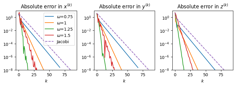
Trial and error shows that the optimum value is \(\omega \approx 1.25\). In this example, the SOR method with this optimum \(\omega\) converges approximately twice as quickly as the Gauss-Seidel method (where \(\omega=1\)).
\(\,\)
Notice that the performance is strongly dependent on the choice of the \(\omega\) parameter. Choosing the best value of \(\omega\) is generally a very hard problem. It is possible to calculate the optimum \(\omega\) for special classes of matrices, but this is beyond the scope of this course. In practice, for general matrices some trial-and-error is used.