Topic 4 - Limits and Series

4.0 Introduction

Limits are very useful throughout mathematics. For instance, the two core concepts of calculus – differentiation and integration – are examples of limits. In this Topic, we’ll look at limits of sequences and limits of functions. We can also consider series, i.e. infinite sums, as being limits of finite sums and we’ll further look at Taylor series, which are very useful in practical applications. For instance, they can be used to approximate functions up to some desired level of accuracy.

Forming limits generally involves some kind of infinite process and so requires a careful handling of the mathematical concept of infinity. It’s important to remember that we can not just use “$\infty$” as though it is an ordinary number and our intuition can sometimes lead us astray. For instance, does it make sense to say “$\infty/\infty=1$”?

Consider the following. Suppose we let a variable $n$ tend to $\infty$, i.e. get larger and larger without bound.

Then surely $n^2$ tends to $\infty$ as well and so the fraction $\dfrac{n^2}{n}$ apparently tends to $\dfrac{\infty}{\infty}$.
But $\dfrac{n^2}{n}=n$ so does that mean $\dfrac{\infty}{\infty}=\infty$?

On the other hand,

the fraction $\dfrac{n}{n^2}$ also apparently tends to $\dfrac{\infty}{\infty}$.
But $\dfrac{n}{n^2}=\dfrac{1}{n}$ which surely tends to $0$ so does that mean $\dfrac{\infty}{\infty}=0$?

Or how about the following?

The fraction $\dfrac{7n}{n}$ also apparently tends to $\dfrac{\infty}{\infty}$.
But $\dfrac{7n}{n}=7$ which surely tends to $7$ so does that mean $\dfrac{\infty}{\infty}=7$?

The point is this fraction “$\infty/\infty$” makes no sense as there is no consistent way of saying what it is. Things like this are sometimes called indeterminates and to handle them, one has to look more closely at what is happening. We will meet some other indeterminates such as “$0/0$”, “$\infty-\infty$”, “$0\times\infty$”, “$1^{\infty}$”,… that have similar bad behaviour and so we will often need to be careful.

4.1 Limits of sequences

Given a sequence of numbers, for example, \[1,\; \frac12\;,\; \frac14\;,\; \frac18\;,\; ...\;,\;\frac{1}{2^n}\;,\;...\] we can ask what happens as $n$ gets very large. In this case, it’s clear that the terms get closer and closer to zero as $n$ increases - we say that the limit of the sequence is $0$. More generally, a sequence $s_1,s_2,s_3,...$ has limit $L$ if $s_n$ gets arbitrarily close to a number $L$ for large enough $n$. (Note as in the above example, the sequence might never actually reach its limit.) We say that $s_n$ tends to $L$ as $n$ tends to infinity, and use the notation
\[\displaystyle\lim_{n\rightarrow\infty}s_n=L\] or alternatively write “$s_n\rightarrow L$ as $n\rightarrow\infty$”.

Examples. $\,$

$(1)\;$ Suppose $s_n=7$ for all $n$, i.e. the constant sequence $7, 7, 7, 7,...$.

Obviously, we should have $s_n\rightarrow 7$ as $n\rightarrow\infty$.

$(2)\;$ Suppose $s_n=1/n$, i.e. the sequence $1, 1/2, 1/3, 1/4,...$.

For large enough $n$, $1/n$ gets arbitrarily small so $1/n\rightarrow 0$ as $n\rightarrow\infty$.

$(3)\;$ Suppose $s_n=(-1)^n$, i.e. the sequence $-1, 1, -1, 1,...$.

This sequence oscillates between $\pm 1$ and doesn’t approach any single number $L$. We say that the limit doesn’t exist.

$(4)\;$ Suppose $s_n=n$, , i.e. the sequence $1, 2, 3, ...$.

Again, this doesn’t approach any given number $L$ (remember $\infty$ is not a number!) and so the limit doesn’t exist. We might however, write $s_n\rightarrow\infty$ as $n\rightarrow\infty$ to signify that the sequence is unbounded.

This is only a rough definition of a limit - what does “arbitrarily close” actually mean? Although we won’t use it much, here is a formal mathematical definition of a limit of a sequence. We say $\displaystyle\lim_{n\rightarrow\infty}s_n=L$ when the following condition holds:

Given $\epsilon>0$, there exists $N$ so that $\;\;|s_n-L|<\epsilon\quad\text{when}\quad n\geq N$.

In other words, given any tolerance $\epsilon>0$, all points $s_n$ are within $\epsilon$ of $L$ from some place onwards in the sequence, depending on $\epsilon$. We can display this by plotting $s_n$ against $n$.

Calculus of Limits Theorem

It’s possible to build up complicated limits from ones we already know (a bit like we do when finding derivatives and integrals using tables of standard ones).

The Calculus of Limits Theorem (COLT) says: Provided that the limits $\displaystyle\lim_{n\rightarrow\infty} s_n=L$ and $\displaystyle\lim_{n\rightarrow\infty} t_n=M$ exist, we have

$\;(i)\;$ $\displaystyle\lim_{n\rightarrow\infty}\;(\lambda s_n)= \lambda L$ for any constant $\lambda$,

$\;(ii)\;$ $\displaystyle\lim_{n\rightarrow\infty}\;(s_n+t_n)= L+M$,

$\;(iii)\;$ $\displaystyle\lim_{n\rightarrow\infty}\;(s_nt_n)= LM$,

$\;(iv)\;$ $\displaystyle\lim_{n\rightarrow\infty}\;(s_n/t_n)= L/M$ provided $M\neq 0$.

It’s important when using this that the original limits $L$ and $M$ do exist.

Examples. $\,$

$(1)\;$ Consider the sequence $s_n=7+\dfrac{1}{n^2}$.

We can just rewrite it using two limits we’ve already seen: \[ \displaystyle\lim_{n\rightarrow\infty} \left(7+\frac{1}{n^2}\right) =\lim_{n\rightarrow\infty}\; 7 +\left(\lim_{n\rightarrow\infty}\;\frac1n\right)^2=7+0^2=7. \]

$(2)\;$ Consider the sequence $s_n=\dfrac{n^2+7n-2}{3n^2+5}$.

Notice the top and bottom both tend to infinity as $n\rightarrow\infty$. However, we can not just substitute $n=\infty$ to get “$\infty/\infty=1$” as that makes no sense. Instead, first divide top and bottom by $n^2$ (the dominant power) as they then do have limits. We can then use COLT to get \[ \lim_{n\rightarrow\infty} s_n= \lim_{n\rightarrow\infty} \frac{1+7/n-2/n^2}{3+5/n^2} =\frac{1+0+0}{3+0}=\frac13. \]

$(3)\;$ Consider the sequence $s_n=\dfrac{n^2}{2n-1}-\dfrac{n^2}{2n+1}$.

Notice each fraction tends to infinity as $n\rightarrow\infty$. However, we can not say the answer is “$\infty-\infty=0$” as again that makes no sense. Maybe try combining the fractions first \[s_n=n^2\left(\frac{1}{2n-1}-\frac{1}{2n+1}\right) =n^2\left(\frac{2}{4n^2-1}\right). \] Again, we can not just say this is “$\infty\times 0$” – that’s another indeterminate and makes no sense. Instead, rewrite as \[s_n=\frac{2n^2}{4n^2-1}=\frac{2}{4-1/n^2}. \] This is in a form we can now apply COLT to and \[ \lim_{n\rightarrow\infty} s_n= \lim_{n\rightarrow\infty} \frac{2}{4-1/n^2}=\frac{2}{4-0}=\frac12.\]

The general trick is to rewrite in a form where COLT can be applied safely.

Squeezing Theorem

As well as COLT, another technique for finding limits using others we already know is the Squeezing theorem (also called the Pinching Theorem): Suppose that \[r_n\leq s_n\leq t_n\] for all (sufficiently large) $n$ and the outer sequences $r_n$, $t_n$ have the same limit, i.e. \[L=\displaystyle\lim_{n\rightarrow\infty} r_n=\displaystyle\lim_{n\rightarrow\infty} t_n\] (and these limits exist). Then $\displaystyle\lim_{n\rightarrow\infty} s_n=L$ as well.

We won’t prove this, but it should be intuitively clear – the sequence $s_n$ is squeezed between two things moving to the same place and there’s nowhere else for it to go. Note for this to work, we need both sides $r_n$ and $t_n$ – you can’t squeeze from one side!

Example. $\,$

Use the Squeezing Theorem to find $\displaystyle\lim_{n\rightarrow\infty} \dfrac{7+\sin(n)}{n}$.

Since $-1\leq \sin(n)\leq 1$ for all $n$, we have \[\dfrac{6}{n}\leq\dfrac{7+\sin(n)}{n}\leq\dfrac{8}{n}\] for all $n$ and the outer sequences both tend to $0$. Hence by squeezing, the middle sequence tends to $0$ as well.

We’ll end the section by looking at a famous limit for the constant $e$.

Example. $\,$

By considering an area under the graph $y=1/x$, one can show that \[\left(1+\frac1n\right)^n\leq e\leq\left(1+\frac1n\right)^{n+1} \qquad\text{for each integer $n\geq 1$.}\] (See the Study Problems.) Now, assuming that $\displaystyle\lim_{n\rightarrow\infty}\left(1+\frac1n\right)^n$ actually exists, we have \[\lim_{n\rightarrow\infty}\left(1+\frac1n\right)^{n+1} =\lim_{n\rightarrow\infty}\left(1+\frac1n\right)\cdot \lim_{n\rightarrow\infty}\left(1+\frac1n\right)^{n} =\lim_{n\rightarrow\infty}\left(1+\frac1n\right)^n.\] That means the two sides of the inequality above have the same limit and the middle sequence (i.e. the constant $e$) is squeezed between them, giving \[e=\lim_{n\rightarrow\infty}\left(1+\frac1n\right)^n.\] This is sometimes used as the definition of the constant $e$. Notice that it is a limit of type “$1^\infty$” and so this is another indeterminate. Similar to “$\infty/\infty$”, we can not just say that it equals $1$.

(Try putting $(1+1/n)^n$ into a calculator for large values of $n$.)

4.2 Limits of functions

Suppose we want to know how a function $f(x)$ behaves as $x$ gets close to a number $a$. Informally, we say $f(x)$ has limit $L$ as $x$ tends to $a$ if $f(x)$ gets arbitrarily close to $L$ when $x$ is sufficiently close (but not equal) to $a$. Note that it doesn’t matter what $f(a)$ is (or if $f(a)$ even exists). We will use the notation \[\displaystyle\lim_{x\rightarrow a}f(x)=L\] or alternatively write “$f(x)\rightarrow L$ as $x\rightarrow a$”.

As with sequences, there is a formal mathematical definition. We say $\displaystyle\lim_{x\rightarrow a}f(x)=L$ if the following condition holds:

Given $\epsilon>0$, there exists $\delta>0$ so that $\quad|f(x)-L|<\epsilon\quad\text{when}\quad 0<|x-a|<\delta$.

In other words, given any tolerance $\epsilon>0$, there is a $\delta$ depending on $\epsilon$ such that $f(x)$ is within $\epsilon$ of $L$ whenever $x$ is within $\delta$ of $a$. In a graph, this means the function $f(x)$ lies in the green box for $a-\delta<x<a+\delta$.

This can be quite hard to work with and takes up a big part of maths courses in Analysis, so we will generally stick with the informal definition: we can make $f(x)$ close to $L$ by making $x$ close (but not equal) to $a$.

Calculus of Limits Theorem

As with limits of sequences, we have a Calculus of Limits Theorem (COLT) for building complicated limits of functions from simple ones we already know.

The Calculus of Limits Theorem (COLT) says: Provided that the limits $\displaystyle\lim_{x\rightarrow a} f(x)=L$ and $\displaystyle\lim_{x\rightarrow a} g(x)=M$ exist, then

$\;(i)\;$ $\displaystyle\lim_{x\rightarrow a} \left(\lambda f(x)\right)= \lambda L$ for any constant $\lambda$,

$\;(ii)\;$ $\displaystyle\lim_{x\rightarrow a} \left(f(x)+g(x)\right)= L+M$,

$\;(iii)\;$ $\displaystyle\lim_{x\rightarrow a} \left(f(x)g(x)\right)= LM$,

$\;(iv)\;$ $\displaystyle\lim_{x\rightarrow a} \left(f(x)/g(x)\right)= L/M$ provided $M\neq 0$.

As in the sequence version, it’s important when using this that $L$ and $M$ do exist.

Examples. $\,$

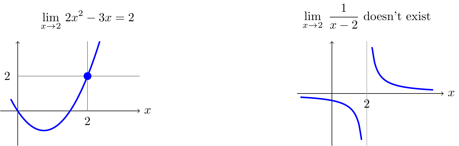
$(1)\;$ Consider the function $f(x)=2x^2-3x$ as $x\rightarrow 2$.

Using the above rules, we can see \[\lim_{x\rightarrow 2}\; f(x)= 2\left(\lim_{x\rightarrow 2}\; x\right)^2 -3\left(\lim_{x\rightarrow 2}\; x\right) =2\times 2^2-3\times 2=2.\]

$(2)\;$ Consider the function $f(x)=\dfrac{x^2+7x-2}{3x^2+5}$ as $x\rightarrow 2$.

As $x\rightarrow 2$, the top tends to $2^2+7\times 2-2=16$ and the bottom tends to $3\times 2^2+5=17$. Since this bottom limit is not zero, we are allowed to divide the limits and find \[\lim_{x\rightarrow 2}\; f(x) =\frac{16}{17}.\]

$(3)\;$ Consider the function $f(x)=\dfrac{1}{x-2}$ as $x\rightarrow 2$.

Don’t just put $x=2$, since that makes the bottom zero and division by zero is bad maths! Instead, notice that $\dfrac{1}{x-2}$ gets arbitrarily large as $x$ gets closer and closer to $2$. Thus $f(x)$ doesn’t approach any particular value $L$ and so the limit doesn’t exist. To indicate that the function is unbounded, we might write $f(x)\rightarrow\infty$ as $x\rightarrow 2$. The graph of $f(x)$ has a vertical asymptote at $x=2$.

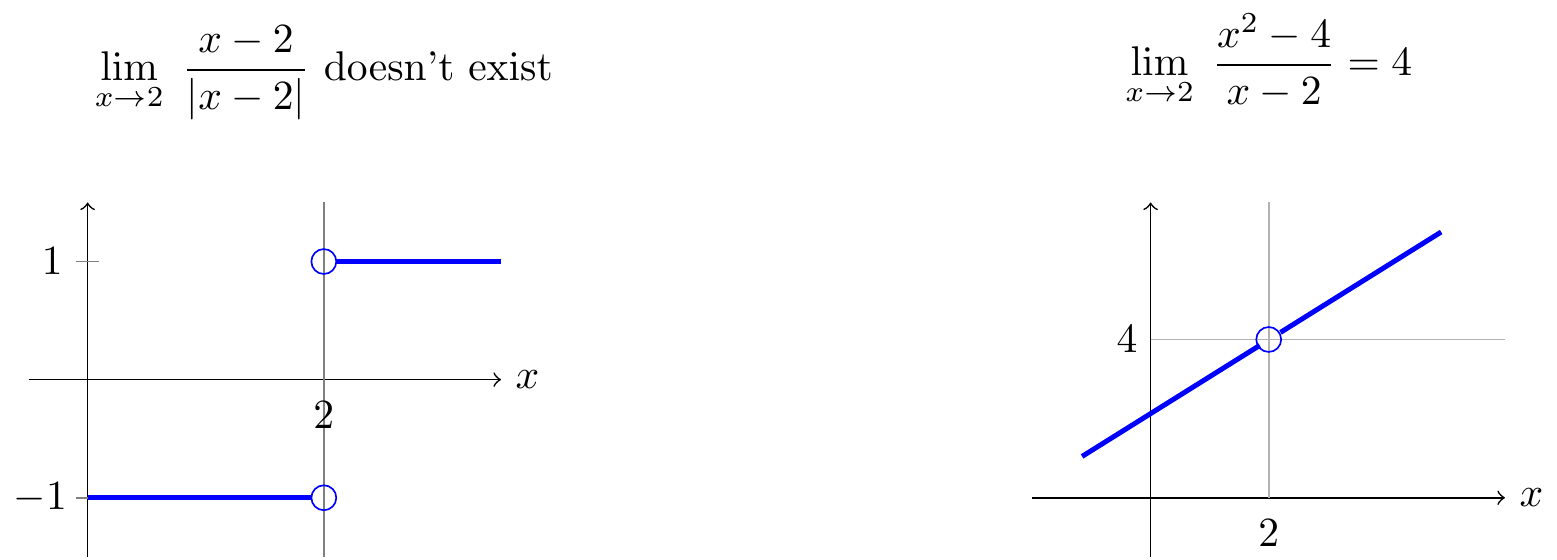
$(4)\;$ Consider the function $f(x)=\dfrac{x-2}{|x-2|}$ as $x\rightarrow 2$.

Again, don’t just put $x=2$ in this since that makes it “$0/0$” which is an indeterminate – just like “$\infty/\infty$”, it can equal anything or nothing!

Instead, notice that $f(x)= \begin{cases} +1\quad\text{if $x>2$,} \\ -1\quad\text{if $x<2$.} \end{cases}$

Thus $f(x)$ doesn’t approach a single value $L$ as $x$ gets close to $2$ and the limit doesn’t exist.

$(5)\;$ Consider the function $f(x)=\dfrac{x^2-4}{x-2}$ as $x\rightarrow 2$.

This time, notice $x^2-4=(x-2)(x+2)$ so $\dfrac{x^2-4}{x-2}=x+2$ as long as $x\neq 2$.

So, for $x$ close but not actually equal to $2$, we find $\dfrac{x^2-4}{x-2}$ gets close to $2+2=4$.

In other words, this limit does exist, even though $f(2)$ doesn’t: \[ \lim_{x\rightarrow 2}\;\frac{x^2-4}{x-2} = \lim_{x\rightarrow 2}\; \frac{(x-2)(x+2)}{x-2}= \lim_{x\rightarrow 2}\; x+2 =2+2=4. \] As with sequences, it often boils down to rewriting the function in a form where COLT can be safely applied.

Squeezing Theorem

As with sequences, there is a Squeezing Theorem for limits of functions: Suppose that \[f(x)\leq g(x)\leq h(x)\] for all $x$ (sufficiently close to $a$) and the outer functions $f(x)$, $h(x)$ have the same limit as $x\rightarrow a$, i.e. \[L=\displaystyle\lim_{x\rightarrow a} f(x)= \displaystyle\lim_{x\rightarrow a} h(x)\] (and these limits exist). Then $\displaystyle\lim_{x\rightarrow a} g(x)=L$ as well.

To demonstrate this in action, we’ll use it (together with a little bit of geometry) to derive an important trigonometric limit.

Example. $\,$ Let’s find $\displaystyle\lim_{x\rightarrow 0}\dfrac{\sin{x}}{x}$. Notice this is a “$0/0$” type limit so it’s not immediately obvious what the answer is – we certainly can’t just substitute $x=0$. Instead, consider some areas in the diagram

area of triangle $ABC$ is $\dfrac12\sin{x}$, since it has base $1$ and height $\sin{x}$,
area of triangle $ABD$ is $\dfrac12\tan{x}$, since it has base $1$ and height $\tan{x}$,
area of shaded sector is $\dfrac12x$, since it is a fraction $x/2\pi$ of the whole circle.

Comparing these areas for any non-zero $x$ between $-\pi/2$ and $\pi/2$, we obtain \[\begin{align*} \frac12\sin{x}\leq \frac12x\leq\frac12\tan{x} &\quad\implies\quad 1\leq \frac{x}{\sin{x}}\leq\frac{1}{\cos{x}} \\ &\quad\implies\quad \cos{x}\leq\frac{\sin{x}}{x}\leq 1. \end{align*}\] Furthermore, since $\displaystyle\lim_{x\rightarrow 0} \cos{x}=\cos(0)=1$, we can apply the squeezing theorem to get \[\lim_{x\rightarrow 0}\;\frac{\sin{x}}{x}=1.\]

Starting from $\displaystyle\lim_{x\rightarrow 0}\;\dfrac{\sin{x}}{x}=1$, we can find various other trigonometric limits.

Examples. $\,$

$(1)\;$ Find $L=\displaystyle\lim_{x\rightarrow\pi}\;\dfrac{\sin{x}}{x-\pi}$.

As $x\rightarrow\pi$, $y=x-\pi\rightarrow 0$, so we can substitute to find \[ L=\lim_{y\rightarrow 0}\;\frac{\sin(y+\pi)}{y}= \lim_{y\rightarrow 0}\;\frac{-\sin{y}}{y}=-1. \]

$(2)\;$ Find $L=\displaystyle\lim_{\theta\rightarrow 0}\;\dfrac{\sin(3\theta)}{\sin\theta}$. We’ll do this in a couple of different ways.

Firstly, recall $\sin(3\theta)=3\sin\theta-4\sin^3\theta$ (from the Complex Numbers topic). Thus, \[ L=\lim_{\theta\rightarrow 0} \;\frac{3\sin\theta-4\sin^3\theta}{\sin\theta} =\lim_{\theta\rightarrow 0}\;\left( 3-4\sin^2\theta\right)=3. \] Alternatively, we have
\[ \frac{\sin(3\theta)}{\sin\theta}=3\left(\frac{\sin(3\theta)}{3\theta}\right) \left(\frac{\sin\theta}{\theta}\right)^{-1} \longrightarrow 3\times 1\times 1^{-1}=3 \] as $\theta\rightarrow 0$, using $\displaystyle\lim_{x\rightarrow 0}\dfrac{\sin{x}}{x}=1$ with $x=3\theta$ and $x=\theta$.

We can also consider the limit $L=\displaystyle\lim_{x\rightarrow\infty}\;f(x)$ of a function $f(x)$ as $x\rightarrow\infty$. By this, we mean that $f(x)$ gets arbitrarily close to $L$ for large enough $x$. (This should look very familiar to the definition of $\displaystyle\lim_{n\rightarrow\infty}s_n$ from the last section and it’s essentially the same, except that $x$ doesn’t have to be an integer as the $n$ did.) On a graph, it means that $f(x)$ has a horizontal asymptote at $L$.

Examples. $\,$

$(1)\;$ Find $L=\displaystyle\lim_{x\rightarrow\infty} \dfrac{x^2+7x-2}{3x^2+5}$.

Don’t just put $x=\infty$, that’s never allowed! Instead, divide top and bottom by $x^2$ (the dominant power) to get \[L=\lim_{x\rightarrow\infty} \frac{1+7/x-2/x^2}{3+5/x^2} =\frac{1+0+0}{3+0}=\frac13.\]

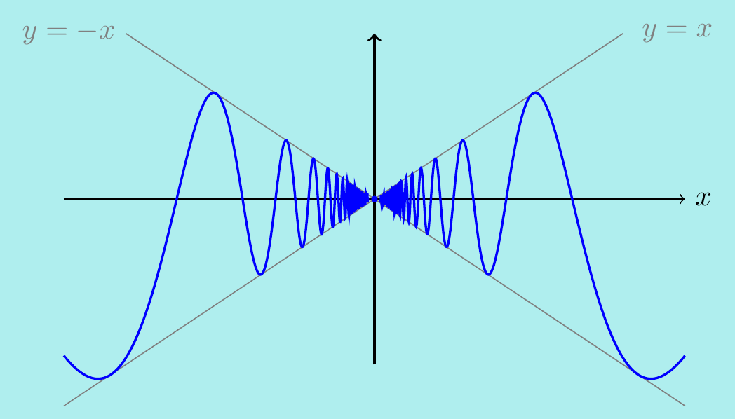
$(2)\;$ Find $L=\displaystyle\lim_{x\rightarrow\infty}\dfrac{\sin{x}}{x}$.

It’s easy to make a mistake here - the answer isn’t $1$! Notice that $-1\leq\sin{x}\leq 1$ so \[-\frac{1}{x}\leq\frac{\sin{x}}{x}\leq\frac{1}{x}.\] These three functions are plotted here.

The two outside terms tend to zero, so by a version of the Squeezing Theorem, the middle does too, i.e. \[L=\displaystyle\lim_{x\rightarrow\infty}\dfrac{\sin{x}}{x}=0.\]

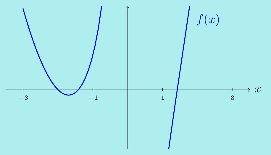
4.3 Continuous functions

One use of limits is to give a mathematical definition of continuity. The intuitive idea of a function being continuous is that we can draw the graph without taking our pen off the paper. Consider the following functions and their limits as $x\rightarrow 2$ discussed in the last section:

The first graph is the only one where we don’t have to lift our pen off the paper when we reach $x=2$. This motivates the following.

Definition$\;$ We say that $f(x)$ is continuous at $x=a$ if $\displaystyle\lim_{x\rightarrow a} f(x)$ exists and equals $f(a)$. Furthermore, a function is called continuous if it is continuous at every point.

For instance, all polynomials are continuous everywhere, as are $e^x$, $\sin{x}$ and $\cos{x}$. However, $\tan{x}$ isn’t continuous at $x=\pi/2$ since $\cos(\pi/2)=0$ and the limit as $x\rightarrow\pi/2$ doesn’t exist. In fact, by COLT, we have the following rules:

If $f(x)$ and $g(x)$ are continuous at $x=a$, then

so is $\lambda f(x)$ for constant $\lambda$,
so is $f(x)+g(x)$,
so is $f(x)g(x)$,
so is $f(x)/g(x)$ provided $g(a)\neq 0$.

Example. $\,$

By the above, we know now that $\dfrac{\sin{x}}{x}$ is continuous everywhere except at $x=0$ where it is undefined.
However, if we define a new function \[f(x)=\begin{cases} \dfrac{\sin{x}}{x} &\quad\text{for $x\neq 0$,} \\[6pt] \;\;\;1 &\quad\text{for $x=0$,} \end{cases}\] then $f(x)$ is continuous everywhere since $\displaystyle\lim_{x\rightarrow 0} f(x)=1=f(0)$. We have essentially removed the discontinuity by adding in the extra point $f(0)=1$ as in the graph below.

As well as sums, products and quotients (as long as we don’t divide by zero) of continuous functions being continuous, another useful fact is that compositions of continuous functions are also continuous: if $g(x)$ is continuous at $a$ and $f(x)$ is continuous at $g(a)$ then $f(g(x))$ is continuous at $a$.

Example. $\,$

The function $\sin(1/x)$ is continuous for $x\neq 0$, since $\sin{x}$ is continuous everywhere and $1/x$ is continuous for $x\neq 0$. However, the limit \[\lim_{x\rightarrow 0}\;\sin\left(\dfrac{1}{x}\right)\] doesn’t exist since we can make $\sin(1/x)$ equal any value between $-1$ and $1$ for arbitrarily small values of $x$. Here’s what the graph looks like:

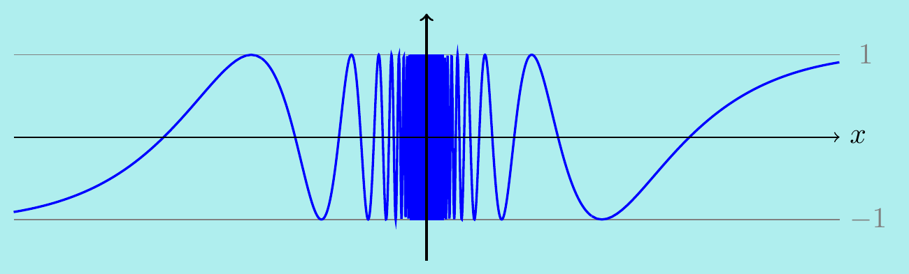
That means there’s no way to modify $\sin(1/x)$ by setting a value at $x=0$ so that it becomes continuous.

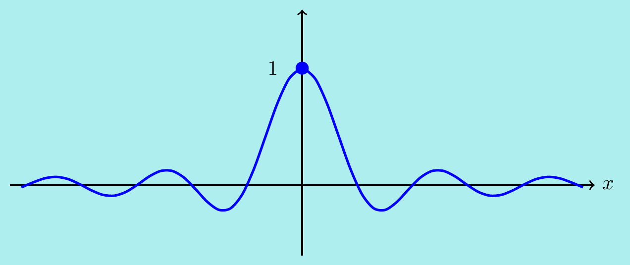
On the other hand, consider \[f(x)=\begin{cases} x\sin\left(\dfrac{1}{x}\right) &\quad\text{for $x\neq 0$,} \\[6pt] \;\;\;0 &\quad\text{for $x=0$.} \end{cases}\] This is a product of functions which are continuous for $x\neq 0$ so it is also continuous there. However, since sine only takes values between $\pm 1$, we have $-x\leq f(x)\leq x$ and so by squeezing, we see that \[\lim_{x\rightarrow 0}\;f(x)=0=f(0).\] This means that $f(x)$ is continuous at $x=0$ as well. Here’s the graph:

Example. $\,$

The function $\;h(x)=\sqrt{\dfrac{x^2+2}{x-1}}\;$ is continuous at all $x>1$.

We have $h(x)=f(g(x))$ where $g(x)=\dfrac{x^2+2}{x-1}$ is continuous for $x\neq 1$ and $f(x)=\sqrt{x}$ is continuous for $x\geq 0$. Notice we need $x>1$ so that we are taking square roots of a positive number $g(x)$.

We can use continuous functions to find some limits of sequences easily via the following fact: suppose that a sequence $s_n\rightarrow L$ as $n\rightarrow\infty$ and $f(x)$ is a continuous function. Then $f(s_n)\rightarrow f(L)$ as $n\rightarrow\infty$.

Example. $\,$

Consider the limit $\;\;\lim_{n\rightarrow\infty} n^2\sin\left(\dfrac{1}{n^2}\right)$.

From the example above, the function \[ f(x)=\begin{cases} \dfrac{\sin{x}}{x} &\quad\text{for $x\neq 0$,} \\[6pt] \;\;\;1 &\quad\text{for $x=0$,} \end{cases} \] is continuous. Now notice if we set $s_n=1/n^2$, then $f(s_n)=n^2\sin\left(\dfrac{1}{n^2}\right)$.

But we know that $s_n=\dfrac{1}{n^2}\rightarrow 0$ as $n\rightarrow\infty$ and so $f(s_n)\rightarrow f(0)=1$ as $n\rightarrow\infty$.

4.4 Differentiable functions

As well, as continuity, limits give us a mathematical way to define differentiation.

The derivative of a function $f(x)$ at a some $x$ is the gradient of the tangent there.

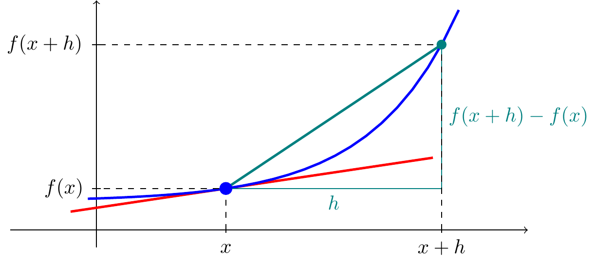
Consider the line joining $\left(x,f(x)\right)$ to $\left(x+h,f(x+h)\right)$. It has gradient
\[\frac{f(x+h)-f(x)}{h}.\] If we let $h$ get smaller and smaller, the line gets closer and closer to the tangent at $x$.

Definition$\;$ We say that $f(x)$ is differentiable at $x$ if the limit \[\lim_{h\rightarrow 0}\;\frac{f(x+h)-f(x)}{h}\] exists, and if that is the case, the limit is called the derivative $f'(x)$. We also sometimes write $\dfrac{df}{dx}=f'(x)$.

Let’s see how this fits with some derivatives we already know.

Example. $\,$

Show that $f(x)=x^2$ is differentiable everywhere and find its derivative.

We have \[\begin{align*} \lim_{h\rightarrow 0}\; \frac{(x+h)^2-x^2}{h} &=\lim_{h\rightarrow 0}\; \frac{2xh+h^2}{h} \\ &=\lim_{h\rightarrow 0}\; 2x+h \\ &=2x. \end{align*}\] In particular, the limit exists for any $x$ and $f'(x)=2x$ as expected.

Example. $\,$

Show that $f(x)=\sin{x}$ is differentiable everywhere and find its derivative.

We can split the limit into parts we can handle, using a double angle formula: \[\begin{align*} \lim_{h\rightarrow 0}\; \frac{\sin(x+h)-\sin(x)}{h} &=\lim_{h\rightarrow 0}\; \frac{\sin{x}\cos(h)+\cos{x}\sin(h)-\sin{x}}{h} \\ &= \cos{x}{\color{maroon}{\left(\lim_{h\rightarrow 0}\; \frac{\sin(h)}{h}\right)}}+ \sin{x}{\color{purple}{\left(\lim_{h\rightarrow 0}\; \frac{\cos(h)-1}{h}\right)}}. \end{align*}\] Now we already know one of these limits: $\;\color{maroon}{\displaystyle\lim_{h\rightarrow 0}\;\dfrac{\sin(h)}{h}=1}$.

For the other, notice \[\begin{align*} \frac{\cos(h)-1}{h} &=\left(\frac{\cos(h)-1}{h}\right)\left(\frac{\cos(h)+1}{\cos(h)+1}\right) \\ &=\frac{\cos^2(h)-1}{h(\cos(h)+1)} \\ &=\left(\frac{\sin(h)}{h}\right)\left(\frac{-\sin(h)}{\cos(h)+1}\right). \end{align*}\] Hence, using COLT with $\;\displaystyle\lim_{h\rightarrow 0}\;\dfrac{\sin(h)}{h}=1\;$ and $\;\displaystyle\lim_{h\rightarrow 0}\;\dfrac{-\sin(h)}{\cos(h)+1}=\frac{0}{1+1}=0,\;$ we get \[{\color{purple}{\lim_{h\rightarrow 0}\;\frac{\cos(h)-1}{h}=0}}.\] Substituting this into the overall limit gives $f'(x)=\cos{x}$, which should be no surprise!

Example. $\,$

Consider the absolute value function \[f(x)=|x|= \begin{cases} x\quad\text{if $x\geq 0$,} \\ -x\quad\text{if $x<0$.} \end{cases}\] It is continuous at $x=0$ by applying squeezing: $|x|$ is squeezed between $-x$ and $x$ and both of these tend to 0 as $x\rightarrow 0$. However, it is not differentiable at $x=0$ since \[\lim_{h\rightarrow 0}\;\frac{f(x+h)-f(x)}{h} =\lim_{h\rightarrow 0}\;\frac{|h|}{h}\] doesn’t exist - it approaches $+1$ for positive $h$ but $-1$ for negative $h$. On the graph of $f(x)=|x|$, there is no well-defined tangent at the origin.

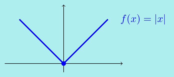
This last example shows that continuous functions are not necessarily differentiable. On the other hand, differentiable functions are automatically continuous.

Indeed, notice by substituting $h=x-a$, the condition for continuity $\displaystyle\lim_{x\rightarrow a}\;f(x)=f(a)$ can be rewritten as \[\lim_{h\rightarrow 0}\;\left[f(a+h)-f(a)\right]=0.\] Now, if $f(x)$ is differentiable at $x=a$, then \[\begin{align*} \lim_{h\rightarrow 0}\;\left[f(a+h)-f(a)\right] &=\lim_{h\rightarrow 0}\left(\frac{f(a+h)-f(a)}{h}\,h\right) \\ &=\left(\lim_{h\rightarrow 0}\frac{f(a+h)-f(a)}{h}\right)\left(\lim_{h\rightarrow 0} h\right) =f'(a)\cdot 0 =0 \end{align*}\] so $f(x)$ is continuous at $a$.

It is immediate from the definition that if a function is constant, say $f(x)=c$ for all $x$, then its derivative vanishes, that is, $f'(x)=0$.

We also have the following familiar rules for computing derivatives: if $f(x)$ and $g(x)$ are differentiable at $x=a$, then

so is $\lambda f(x)$ for constant $\lambda$, and we have $\dfrac{d}{dx}(\lambda f(x))=\lambda f'(x)$,
so is $f(x)+g(x)$, and we have $\dfrac{d}{dx}(f(x)+g(x))=f'(x)+g'(x)$,
so is $f(x)g(x)$, and we have the product rule \[\frac{d}{dx}\left(f(x)g(x)\right)=f'(x)g(x)+f(x)g'(x),\]
so is $f(x)/g(x)$ provided $g(a)\neq 0$, and we have the quotient rule \[\frac{d}{dx}\left(\frac{f(x)}{g(x)}\right)=\frac{f'(x)g(x)-f(x)g'(x)}{g(x)^2}.\]

Another useful property is the chain rule, which tells us about compositions:

If $g(x)$ is differentiable at $x=a$ and $f(x)$ is differentiable at $x=g(a)$, then $f(g(x))$ is differentiable at $x=a$ and \[ \frac{d}{dx}\left(f(g(x)\right) =f'\left(g(x)\right)g'(x). \] Letting $y=f(u)$ and $u=g(x)$, the chain rule can be written in the suggestive form \[\dfrac{dy}{dx}=\dfrac{dy}{du}\cdot\dfrac{du}{dx}\]

These rules can all be proved directly using the definition of differentiation as a limit, together with COLT, though (iii), (iv) and (v) get a bit tricky. For instance, here’s how to prove the product rule: we have to find the limit as $h\rightarrow 0$ of \[\begin{align*} \frac{f(x+h)g(x+h)-f(x)g(x)}{h} =\left(\frac{f(x+h)-f(x)}{h}\right)g(x+h) +f(x)\left(\frac{g(x+h)-g(x)}{h}\right). \end{align*}\] Now \[\lim_{h\rightarrow 0}\;\frac{f(x+h)-f(x)}{h}=f'(x),\quad \lim_{h\rightarrow 0}\;\frac{g(x+h)-f(x)}{h}=g'(x)\] and $\displaystyle\lim_{h\rightarrow 0}\;g(x+h)=g(x)$, since $g(x)$ is differentiable hence continuous.

Putting this altogether using COLT, the overall limit is $f'(x)g(x)+f(x)g'(x)$ as required.

4.5 Intermediate and Extreme values

Intermediate Values

A very natural, useful consequence of the definition of continuity is the following:

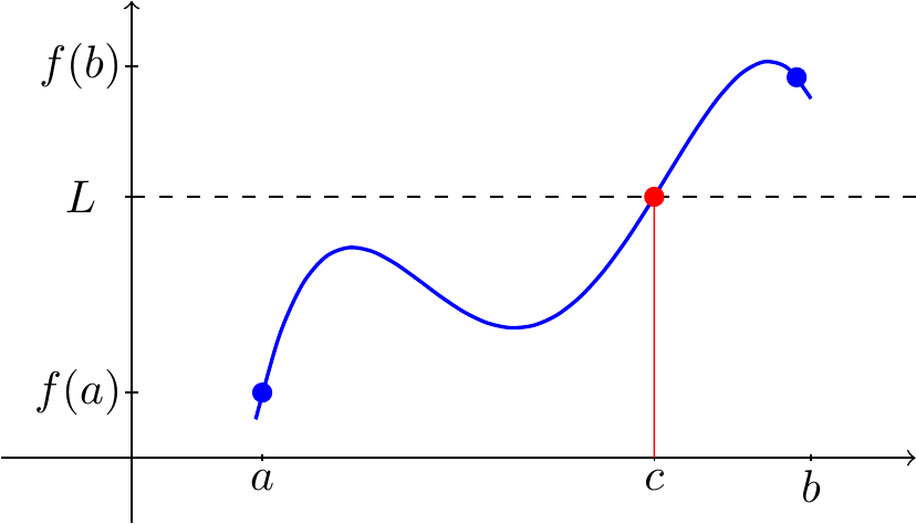
The Intermediate Value Theorem$\;$ Suppose $f(x)$ is continuous between $a$ and $b$ and $L$ lies between $f(a)$ and $f(b)$. Then $f(c)=L$ for some $c$ between $a$ and $b$.

We won’t prove this but just note what it says: any horizontal line between $y=f(a)$ and $y=f(b)$ intersects the graph $y=f(x)$ in at least one place. In other words, continuous functions don’t miss any intermediate values and the graph is an “unbroken curve”.

We can use this to locate solutions to $f(x)=0$ - look for where $f(x)$ changes sign.

Example. $\,$

Where does $f(x)=x^2+2x-2-\dfrac{4}{x}=0$? Note $f(x)$ is continuous everywhere except $x=0$ so let’s look for where it changes sign:

We have $f(1)=-3<0$ and $f(3)=\frac{35}{3}>0$ and so by the theorem there must be a root, i.e. a solution to $f(x)=0$ in the interval $-1<x<3$.
We have $f(-1)=1>0$ and $f(1)=-3<0$. However we cannot conclude there is a root in $-1<x<1$ as $f(x)$ is not continuous on that interval. In fact there are no roots here.
We have $f(-3)=\frac{7}{3}>0$ and $f(-1)=1>0$ so can make no immediate conclusion about roots in the interval $-3<x<-1$. Checking further points in the interval would reveal two roots.

Actually, one can check $f(x)=\dfrac{(x+2)(x^2-2)}{x}$ so $f(x)=0$ precisely when $x=-2,\pm\sqrt{2}$.

One can extend the idea (by repeatedly halving the intervals) to give a simplistic algorithm (the bisection method) for approximating solutions. We’ll see a generally better way of finding approximate solutions later in this topic.

Extreme Values

One of the things we often use derivatives for is to find extreme values of functions, i.e. turning points on a graph. Let’s check that our limit definition does this as one would hope. We say that $f(x)$ has

a local minimum at $x=a$ if $f(a)\leq f(a+h)$ for sufficiently small $h$,
a local maximum at $x=a$ if $f(a)\geq f(a+h)$ for sufficiently small $h$.

Extreme Value Theorem$\;$ Suppose $f(x)$ is differentiable at $x=a$ and has a local minimum or local maximum at that point. Then $f'(a)=0$.

To indicate why this is true, notice if $f(x)$ is differentiable at $x=a$ then the limit
\[f'(a)=\lim_{h\rightarrow 0} \frac{f(a+h)-f(a)}{h}\] exists. But if $f(x)$ has a local minimum at $x=a$ then \[\frac{f(a+h)-f(a)}{h}\quad\text{is}\quad \begin{cases} \geq 0 \quad\text{if $h>0$} \\ \leq 0 \quad\text{if $h<0$} \end{cases}\] so the only way the limit can exist is if it is zero, i.e. $f'(a)=0$.

A similar argument will show the same for a local maximum. By looking more closely, one can obtain the usual second derivative test for maximal and minimal values:

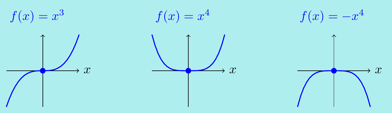
Suppose that $f(x)$ is twice differentiable at $a$. Then

if $f'(a)=0$ and $f''(a)>0$ then $f(x)$ has a local minimum at $x=a$,
if $f'(a)=0$ and $f''(a)<0$ then $f(x)$ has a local maximum at $x=a$.
if $f'(a)=f''(a)=0$ then no conclusion can be made (without more information).

Example. $\,$

The third case here really is inconclusive – it does not mean there is a point of inflection. Notice each of the following satisfy $f'(0)=f''(0)=0$ and have a point of inflection, a local minimum and local maximum respectively:

Later this term we will see a version of the second derivative test for functions of two variables $f(x,y)$ and use it to find extreme points on surfaces rather than curves.

4.6 L’Hôpital’s Rule

We can use differentiation to find more limits.

L’Hôpital’s Rule (“$0/0$” form):$\;$ Suppose $f(x)$ and $g(x)$ are differentiable functions where $f(x)\rightarrow 0$ and $g(x)\rightarrow 0$ as $x\rightarrow a$ and $g'(x)\neq 0$ in the approach. If $L=\displaystyle\lim_{x\rightarrow a}\frac{f'(x)}{g'(x)}$ exists, then $\displaystyle\lim_{x\rightarrow a}\frac{f(x)}{g(x)}=L$ as well.

We’ll give a sketch proof in the particular case $f(a)=g(a)=0$ and $g'(a)\neq 0$.

Using that $f(a)=g(a)=0$, in terms of $h=x-a$ we have \[ \lim_{x\rightarrow a}\;\frac{f(x)}{g(x)} =\lim_{x\rightarrow a}\;\frac{f(x)-f(a)}{g(x)-g(a)} =\lim_{h\rightarrow 0}\;\frac{f(a+h)-f(a)}{g(a+h)-g(a).} \] As $f$ and $g$ are differentiable at $x=a$ and $g'(a)\neq0$, the last expression can be computed as \[ \displaystyle\lim_{h\rightarrow 0}\;\dfrac{\dfrac{f(a+h)-f(a)}{h}} {\dfrac{g(a+h)-g(a)}{h}} =\dfrac{\displaystyle\lim_{h\rightarrow 0}\;\frac{f(a+h)-f(a)}{h}} {\displaystyle\lim_{h\rightarrow 0}\;\frac{g(a+h)-g(a)}{h}}=\frac{f'(a)}{g'(a)}. \]

L’Hôpital’s Rule makes finding some limits very easy, as long as we are good at differentiation.

Examples. $\,$ $(1)\;$ We immediately get the famous limit \[\lim_{x\rightarrow 0}\;\frac{\sin{x}}{x}= \lim_{x\rightarrow 0}\frac{\cos{x}}{1}=1.\] (Note the amusing circularity in our logic though! We need to know the derivative of $\sin{x}$ to do this, but to show that $\frac{d}{dx}\sin{x}=\cos{x}$, we used the limit $\lim_{x\rightarrow 0}\frac{\sin{x}}{x}=1$. )

$(2)\;$ We can also apply l’Hôpital’s Rule multiple times if we keep getting “0/0” type limits: \[\begin{align*} \lim_{x\rightarrow 0}\;\frac{\sin{x}-x}{x^3} =\lim_{x\rightarrow 0}\;\frac{\cos{x}-1}{3x^2} =\lim_{x\rightarrow 0}\;\frac{-\sin{x}}{6x} =\lim_{x\rightarrow 0}\;\frac{-\cos{x}}{6}=-\frac16. \end{align*}\]

$(3)\;$ However, you must be careful – as with any powerful tool, careless application can cause trouble. For instance, what is wrong with the following? \[\lim_{x\rightarrow 0}\;\frac{\cos{x}}{x}= \lim_{x\rightarrow 0}\frac{-\sin{x}}{1}=0.\] This is certainly wrong. If $0<x<\dfrac{\pi}{3}$, then $\cos{x}>\dfrac12$ and so $\dfrac{\cos{x}}{x}>\dfrac{1}{2x}$ which is unbounded as $x\rightarrow 0$. The error was to apply l’Hôpital’s Rule to a limit of the form “$1/0$”, which behaves very differently.

For this reason, you should always check and explicitly say that the top and bottom both tend to $0$. You should also explicitly say when you are using l’Hôpital’s Rule. (You will lose marks in the exam if you don’t!)

There are other ways that l’Hôpital’s Rule can be applied. For instance, it works for a ``$0/0$’’ limit when $x\rightarrow\infty$ too:

Example. $\,$ Find $L=\displaystyle\lim_{x\rightarrow\infty}\;x\left(e^{2/x}-1\right)$.

Rewriting it in the form $\displaystyle\lim_{x\rightarrow\infty}\;\dfrac{e^{2/x}-1}{1/x}$, it is now of the form “$0/0$” and l’Hôpital’s Rule applies. Differentiating top and bottom gives \[L=\lim_{x\rightarrow\infty}\;\frac{e^{2/x}(-2/x^2)}{-1/x^2} =\lim_{x\rightarrow\infty}\; 2e^{2/x}=2e^0=2.\]

It’s also possible to turn L’Hôpital’s Rule on its head to handle limits of the form “$\infty/\infty$”.

L’Hôpital’s Rule (“$\infty/\infty$” form):$\;$ Suppose $f(x)$ and $g(x)$ are differentiable functions with $f(x)\rightarrow \pm\infty$ and $g(x)\rightarrow \pm\infty$ as $x\rightarrow a$ and $g'(x)\neq 0$ in the approach. If $L=\displaystyle\lim_{x\rightarrow a}\frac{f'(x)}{g'(x)}$ exists, then $\displaystyle\lim_{x\rightarrow a}\frac{f(x)}{g(x)}=L$ as well.

(Again, this works for $x\rightarrow\infty$ too.)

Example. $\,$ Find $L=\displaystyle\lim_{x\rightarrow\infty}\;\dfrac{\ln{x}}{x^2}$.

This is of the form “$\infty/\infty$” and l’Hôpital’s Rule applies. Differentiating top and bottom gives \[L=\lim_{x\rightarrow\infty}\;\frac{1/x}{2x}= \lim_{x\rightarrow\infty}\;\frac{1}{2x^2}=0.\]

A final interesting example is

Example. $\,$ Find $L=\displaystyle\lim_{x\rightarrow\infty}\;\left(1+\dfrac{1}{x}\right)^x$.

Let $f(x)=x\ln\left(1+\frac{1}{x}\right)$. Then $L=\displaystyle\lim_{x\rightarrow\infty}\;e^{f(x)}= e^{\lim_{x\rightarrow\infty}\; f(x)}$ as $e^x$ is a continuous function. However, \[\begin{align*} \lim_{x\rightarrow\infty}\;f(x)= \lim_{x\rightarrow\infty}\; x\ln\left(1+\frac{1}{x}\right) &= \lim_{u\rightarrow 0}\; \frac{\ln(1+u)}{u} \end{align*}\] by putting $u=1/x$. We can now use l’Hôpital’s Rule for this “$0/0$” limit to find \[\lim_{u\rightarrow 0}\; \frac{\ln(1+u)}{u} =\lim_{u\rightarrow 0}\; \frac{1/(1+u)}{1}=1\] and so $L=e^1=e$.

Using the same ideas, one can actually define $e^t$ for any $t$ by a limit, similarly to how we did for $e$: \[e^t=\lim_{n\rightarrow\infty}\;\left(1+\dfrac{t}{n}\right)^n.\]

4.7 Leibniz’s Rule

Recall the product rule for differentiation: $\;\;(uv)'=u'v+uv'.$

What happens if we differentiate again? \[\begin{align*} (uv)''&= \left[u''v+u'v'\right]+\left[u'v'+uv''\right] \\ &=u''v+2u'v'+uv''. \end{align*}\] And again? \[\begin{align*} (uv)'''&= \left[u'''v+u''v'\right]+2\left[u''v'+u'v''\right]+\left[u'v'+uv'''\right] \\ &=u'''v+3u''v'+3u'v''+uv'''. \end{align*}\] Notice the coefficients $1,1$ and $1,2,1$ and $1,3,3,1$ are rows of Pascal’s triangle, i.e. the binomial coefficients \[\displaystyle\binom{n}{m}=\frac{n!}{m!(n-m)!}.\] This pattern continues (and can be proved by induction), giving a formula $n$th derivative of a product.

Write a superscript $u^{(m)}$ to indicate the $m$th derivative of a function $u$. Then Leibniz’s Rule says \[\begin{multline*} (uv)^{(n)}=u^{(n)}v+\binom{n}{1}u^{(n-1)}v^{(1)}+\binom{n}{2}u^{(n-2)}v^{(2)}+... \\ ...+\binom{n}{n-2}u^{(2)}v^{(n-2)}+\binom{n}{n-1}u^{(1)}v^{(n-1)}+uv^{(n)}. \end{multline*}\]

Examples. $\,$ Find the 4th derivatives of $\;\;(i)\;\;e^x\sin{x}\;\;$ and $\;\;(ii)\;\;x^2\ln{x}$.

Leibniz’s Rule for the 4th derivative says \[(uv)''''=u''''v+4u'''v'+6u''v''+4u'v'''+uv''''.\] $(i)\;$ Setting $u(x)=e^x$ and $v(x)=\sin{x}$, we get \[\begin{align*} \frac{d^4}{dx^4}\;\left(e^x\sin{x}\right) &= e^x\sin{x}+4e^x\cos{x}+6e^x(-\sin{x})+4e^x(-\cos{x})+e^x\sin{x} \\ &= -4e^x\sin{x}. \end{align*}\]

$(ii)\;$ Setting $u(x)=x^2$ and $v(x)=\ln{x}$, we get: \[\begin{align*} \frac{d^4}{dx^4}\;\left(x^2\ln{x}\right) &= \left(0\right)\left(\ln{x}\right) +4\left(0\right)\left(\frac1x\right) +6\left(2\right)\left(-\frac{1}{x^2}\right) +4\left(2x\right)\left(\frac{2}{x^3}\right) +\left(x^2\right)\left(-\frac{6}{x^4}\right) \\ &= -\frac{2}{x^2}. \end{align*}\]

Notice the formal similarity with the Binomial Theorem: \[\begin{multline*} (x+y)^n=x^n+\binom{n}{1}x^{n-1}y+\binom{n}{2}x^{n-2}y^2+\,... \\ \ldots\,+\binom{n}{n-2}x^2y^{n-2}+\binom{n}{n-1}xy^{n-1}+y^{n}. \end{multline*}\] In Leibniz’s Rule, however, it is important to write e.g. $v^{(m)}$ and not $v^m$. These are different things - one is a power and the other is a derivative. In particular, the zero-th derivative of a function is $v^{(0)}=v$ and not $v^0=1$, which is why the formula in Leibniz’s Rule starts $\;u^{(n)}v+...$

4.8 The Newton-Raphson Method

The subject of Numerical Analysis includes many algorithms and iterative methods for finding approximate solutions to equations and we’ve already seen a few methods for simultaneous linear equations.

The Newton-Raphson method is a very effective iteration for estimating numerical solutions to any equation $f(x)=0$, as long as we can differentiate $f$.

Suppose we start with an approximate solution $x_0$. The idea is to draw the tangent line to the function at $x_0$ and find the point $x_1$ where this intersects the $x$-axis. Then hopefully $x_1$ should be a better approximation to the actual solution $x$.

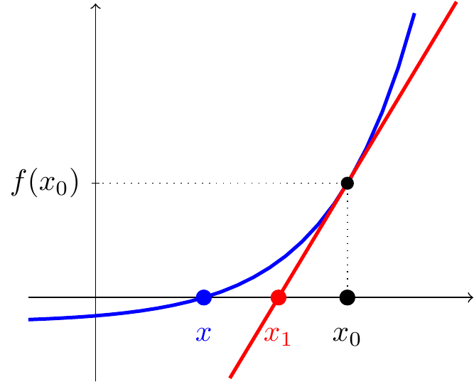
The gradient of the tangent is $f'(x_0)$ so this tangent line has equation \[y-f(x_0)=f'(x_0)(x-x_0).\] This crosses the $x$-axis when $y=0$, hence \[0-f(x_0)=f'(x_0)(x_1-x_0),\] that is, \[x_1=x_0-\frac{f(x_0)}{f'(x_0)}.\]

We are effectively approximating the function with a degree 1 polynomial, i.e. approximating the graph with the tangent line \[f(x)\approx f(x_0)+f'(x_0)(x-x_0).\] In the next sections, we’ll see how Taylor polynomials give us similar approximations of $f(x)$ using higher degree polynomials.

Now that we have a better solution $x_1$, we can repeat to find an even better one $x_2$ and so on, using the iteration \[\boxed{x_{n+1}=x_n-\frac{f(x_n)}{f'(x_n)}.}\] This is the Newton-Raphson Method.

Example. $\,$ Approximate $\sqrt3$ correct to 4 significant figures.

We want to solve $f(x)=x^2-3=0$. Since $f(1)=-2$ and $f(2)=1$, the graph must cross the $x$-axis somewhere between $1$ and $2$ (using the Intermediate Value Theorem, since $f(x)$ is evidently continuous).

Let’s start with initial guess $x_0=2$. Then, using $f'(x)=2x$,
\[\begin{align*} x_1&=x_0-\frac{f(x_0)}{f'(x_0)}=2-\frac{2^2-3}{2\times 2}=\frac{7}{4}\approx 1.7500 \\ x_2&=x_1-\frac{f(x_1)}{f'(x_1)} =\frac74-\frac{\left(\frac74\right)^2-3}{2\times\frac74}=\frac{97}{56}\approx 1.7321 \\ x_3&=x_2-\frac{f(x_2)}{f'(x_2)} =1.7321-\frac{1.7321^2-3}{2\times 1.7321}\approx 1.7321 \end{align*}\] All further iterations will give the same result so we obtain $\sqrt3\approx 1.732$.

Checking $1.732^2=2.999824$ shows this is very close to the actual solution and, as a bonus, we get the fractional approximation $\sqrt3\approx\dfrac{97}{56}$.

Example. $\,$ Find the solution to $e^x+x=2$, correct to 3 decimal places.

First, put this in the correct form $f(x)=0$ with $f(x)=e^x+x-2$.

Notice $f(0)=-1$, $f(1)=e-1>0$ so there must be a solution between $0$ and $1$.

Actually, since $f'(x)=e^x+1>0$, the function is increasing so there is exactly one solution.

Let’s start with $x_0=0$. Then, \[\begin{align*} x_1&=x_0-\frac{f(x_0)}{f'(x_0)}=0-\frac{1+0-2}{1+1}=\frac{1}{2}\approx 0.5000 \\ x_2&=x_1-\frac{f(x_1)}{f'(x_1)} =\frac12-\frac{e^{1/2}+\frac12-2}{e^{1/2}+1}\approx 0.4439 \\ x_3&=x_2-\frac{f(x_2)}{f'(x_2)} =0.4439-\frac{e^{0.4439}+0.4439-2}{e^{0.4439}+1}\approx 0.4429 \\ x_4&\approx 0.4429 \end{align*}\] The iteration has stabilised and the answer is $x\approx 0.443$ to 3 decimal places.

The Newton-Raphson Method is usually very good. In fact, under the right conditions, it converges quadratically, which means that the number of correct significant figures practically doubles after each iteration. This is significantly faster than the bisection method mentioned in Section 4.5.

Unfortunately, the Newton-Raphson doesn’t always work so well. Let’s think about some of the ways it could go wrong:

Clearly, we need $f(x)$ to be differentiable since we need to calculate its derivative!
If we accidentally choose $x_0$ badly so that $f'(x_n)=0$ for some $n$ then the formula will fail since we would have to divide by zero.
We can also accidentally get trapped in a cycle - for instance, it’s possible for $x_0$ to lead to $x_1$ which then leads back to $x_2=x_0$. For instance, consider $f(x)=x^3-2x+2$ with initial guess $x_0=1$.
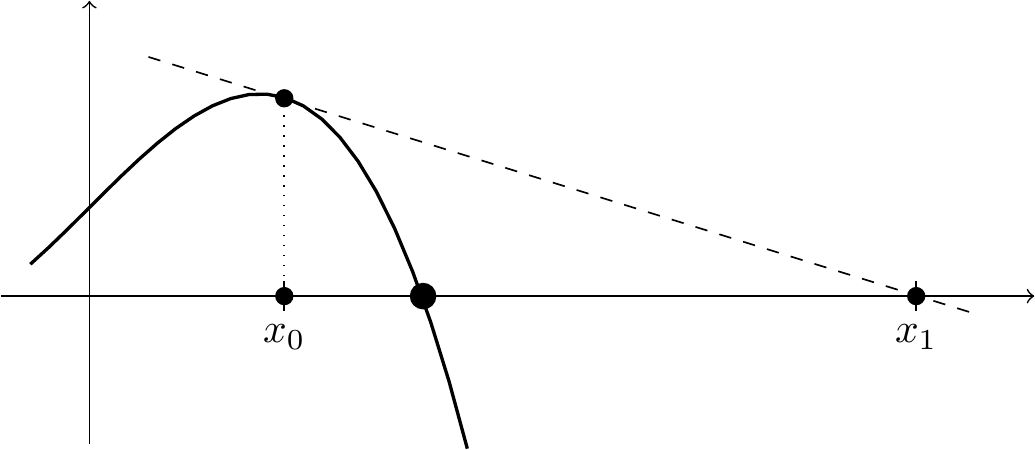
Another thing that can go wrong is if $f(x)=0$ has more than one solution. We might want one in particular but it’s possible that the Method converges to the wrong one. For instance, with $f(x)=2x^3-4x^2+1$, starting from $x_0=1$ leads to a solution $x\approx 0.5970$ but starting from $x_0=2$ leads to another solution $x\approx 1.855$. In practice, one needs to start sufficiently close to the solution you are trying to estimate.
Yet another way it might not work well is if $f'(x_0)$ is very close to 0. That means the tangent will be close to horizontal and $x_1$ can be further away from the exact solution than $x_0$. And then $x_2$ could be even further away and so forth.

4.9 Taylor Series introduction

The idea behind Taylor series starts with approximating a function by polynomials of higher and higher degrees.

We have seen that $\displaystyle\lim_{x\rightarrow0}\;\dfrac{\sin{x}}{x}=1$, so that for very small $x$, we have a pretty good approximation \[\sin{x}\approx x.\]

We also saw, via l’Hôpital’s Rule, that $\displaystyle\lim_{x\rightarrow0}\;\dfrac{\sin{x}-x}{x^3}=-\dfrac16$, so by re-arranging, we get a better approximation \[\sin{x}\approx x-\frac16x^3.\] If we continued to find better and better polynomial approximations, we’d end up with \[\sin{x}\approx x-\frac{x^3}{3!}+\frac{x^5}{5!}-\frac{x^7}{7!}+... +(-1)^k\frac{x^{2k+1}}{(2k+1)!}.\] This sum is an example of a Taylor polynomial and by taking more and more terms (i.e. looking at the limit as $k\rightarrow\infty$), we obtain an infinite sum which actually equals $\sin{x}$ for all $x$: \[\sin{x}=x-\frac{x^3}{3!}+\frac{x^5}{5!}-\frac{x^7}{7!}+... +(-1)^k\frac{x^{2k+1}}{(2k+1)!}+...\] This is a Taylor series. (It is a special case of a power series - infinite sums of multiples of powers.)

More generally, a Taylor series about $x=a$ is an infinite sum of the form \[f(x)=c_0+c_1(x-a)+c_2(x-a)^2+c_3(x-a)^3+...+c_n(x-a)^n+...\]

Suppose we have such a sum. Then, by repeatedly differentiating and setting $x=a$ we can find the coefficients $c_0, c_1, c_2,...$ in terms of $f$. \[\begin{align*} f(x)&=c_0+c_1(x-a)+c_2(x-a)^2+c_3(x-a)^3+... \hspace{-1cm}&\implies\quad f(a)&=c_0 \\ f'(x)&=c_1+2c_2(x-a)+3c_3(x-a)^2+... \hspace{-1cm}&\implies\quad f'(a)&=c_1 \\ f''(x)&=2c_2+6c_3(x-a)+... \hspace{-1cm}&\implies\quad f''(a)&=2c_2 \\ f'''(x)&=6c_3+... \hspace{-1cm}&\implies\quad f'''(a)&=6c_3 \end{align*}\] and generally, $f^{(n)}(a)=n!c_n$. In other words, the above formula can be written as: \[\begin{multline*} f(x)=f(a)+f'(a)(x-a)+\frac{f''(a)}{2!}(x-a)^2+\frac{f'''(a)}{3!}(x-a)^3+... \\ ...+\frac{f^{(n)}(a)}{n!}(x-a)^n+... \end{multline*}\]

Under certain conditions, we will find that this infinite sum does actually converge to $f(x)$ for appropriate values of $x$. We’ll return to this issue later, but for now, just assume these series make sense. If we stop at the $(x-a)^n$ term, we get the degree $n$ Taylor polynomial of $f(x)$ about $x=a$. This is written as \[\begin{multline*} P_{n,a}(x)=f(a)+f'(a)(x-a)+\frac{f''(a)}{2!}(x-a)^2+\frac{f'''(a)}{3!}(x-a)^3+...\\ ...+\frac{f^{(n)}(a)}{n!}(x-a)^n \end{multline*}\] and the Taylor series (if it exists) is the limit as $n\rightarrow\infty$ of these: \[f(x)=\lim_{n\rightarrow\infty} P_{n,a}(x).\]

Example. $\,$ Find the Taylor series of $f(x)=e^x$ about $x=0$.

We have $f^{(n)}(x)=e^x$ for all $n$ so $f^{(n)}(0)=e^0=1$. The Taylor polynomial is just \[P_{n,0}(x)=1+x+\frac{x^2}{2!}+\frac{x^3}{3!}+...+\frac{x^n}{n!}.\] If we forget to stop at $x^n$, then we get the Taylor series for $e^x$ about $x=0$: \[e^x=1+x+\frac{x^2}{2!}+\frac{x^3}{3!}+...+...+\frac{x^n}{n!}+...\]

You could actually take this as the definition of $e^x$ for any $x$. We already saw an alternative definition \[e^x=\lim_{n\rightarrow\infty}\;\left(1+\frac{x}{n}\right)^n\] and showing these two expressions for $e^x$ are actually equal is doable but quite tricky.

Example. $\,$ Find the Taylor series of $f(x)=\sin{x}$ about $x=0$.

We’ll do it in two ways. First, notice that the derivatives just cycle through $\sin{x}$, $\cos{x}$, $-\sin{x}$, $-\cos{x},...$ so actually $f^{(n)}(0)$ cycles through the values $0,1,0,-1,0,1,0,-1,...$

This could be written as \[f^{(n)}(0)=\begin{cases} 0 &\qquad\text{if $n$ is even} \\ (-1)^{\frac{n-1}{2}} &\qquad\text{if $n$ is odd} \end{cases}\] In particular, we recover the Taylor series from the beginning of the section: \[\sin{x}=x-\frac{x^3}{3!}+\frac{x^5}{5!}-\frac{x^7}{7!}+...\]

Alternatively, we can do a neat trick with complex numbers. Swap $x$ with $ix$ in the Taylor series for $e^x$: \[\begin{align*} e^{ix}&=1+ix+\frac{(ix)^2}{2!}+\frac{(ix)^3}{3!}+\frac{(ix)^4}{4!}+... \\ &= 1+ix-\frac{x^2}{2!}-i\frac{x^3}{3!}+\frac{x^4}{4!}+... \\ &=\left(1-\frac{x^2}{2!}+\frac{x^4}{4!}-...\right) +i\left(x-\frac{x^3}{3!}+\frac{x^5}{5!}-...\right) \\ &=\cos{x}+i\sin{x} \end{align*}\] The imaginary part gives us the Taylor series for $\sin{x}$ and we simultaneously find the Taylor series for $\cos{x}$ by looking at the real part: \[\cos{x}=1-\frac{x^2}{2!}+\frac{x^4}{4!}-\frac{x^6}{6!}+...\]

A Taylor series about $x=0$ is sometimes called a Maclaurin series. In fact, when we talk about a Taylor series without specifying it is about $x=a$, by convention we mean the Taylor series about $x=0$. Sometimes however, we don’t want to or can’t expand in powers of $x$ and the more general case is useful.

Example. $\,$ The Taylor series for $f(x)=e^x$ about $x=a$ is \[\begin{align*} e^x&=f(a)+f'(a)(x-a)+\frac{f''(a)}{2!}(x-a)^2+\frac{f'''(a)}{3!}(x-a)^3+... \\ &=e^a+e^a(x-a)+\frac{e^a}{2!}(x-a)^2+\frac{e^a}{3!}(x-a)^3+... \end{align*}\] Notice if $x$ is close to $a$, the powers $(x-a)^n$ will get small very quickly so we would expect the Taylor polynomials should give good approximations to $e^x$ for $x$ close to $a$. For instance, we find the parabola \[y=e^2+e^2(x-2)+\frac12e^2(x-2)^2\] is close to $y=e^x$ when $x$ is close to $2$.

Example. $\,$ Find the Taylor series for $f(x)=\ln{x}$ about $x=0$.

This breaks immediately - we need to substitute in $f(0)$ but this is infinite. A better question is: find the Taylor series for $f(x)=\ln(1+x)$ about $x=0$.

We have $f(x)=\ln(1+x)$, $f'(x)=(1+x)^{-1}$, $f''(x)=-(1+x)^{-2}$, $f'''(x)=2(1+x)^{-3},...$

and generally, $f^{(n)}(x)=(-1)^{n-1}(n-1)!(1+x)^{-n}$ for $n\geq 1$.

Hence the Taylor series is \[\begin{align*} \ln(1+x)&=f(0)+f'(0)x+\frac{f''(0)}{2!}x^2+\frac{f'''(0)}{3!}x^3+... \\ &=0+x-\frac{1!}{2!}x^2+\frac{2!}{3!}x^3-\frac{3!}{4!}x^3+... \\ &=x-\frac{x^2}{2}+\frac{x^3}{3}-\frac{x^4}{4}+... \end{align*}\]

4.10 Convergence and Taylor’s Theorem

We now come to the matter of convergence of Taylor series as the limit of the Taylor polynomials $P_{n,a}(x)$ as $n\rightarrow\infty$.

Let’s first look at a special case with the function $f(x)=\dfrac{1}{1-x}$ about $x=0$. We have \[f'(x)=\frac{1}{(1-x)^2},\quad f''(x)=\frac{2}{(1-x)^3},\quad f'''(x)=\frac{6}{(x-1)^4},\;\;...\] and generally $f^{(n)}(0)=n!$ so the degree $n$ Taylor polynomial of $f(x)$ about $x=0$ is \[P_{n,0}(x)=1+x+x^2+...+x^n.\] This is a geometric sum and (provided $x\neq 1$), can be written \[\begin{align*} P_{n,0}(x)=\frac{1-x^{n+1}}{1-x}=f(x)-\frac{x^{n+1}}{1-x}. \end{align*}\]

Hence the remainder term, i.e. the difference between $f(x)$ and $P_{n,0}(x)$ is \[R_n(x)=f(x)-P_{n,0}(x)=\frac{x^{n+1}}{1-x}.\] But notice that for $|x|<1$, this tends to 0 as $n\rightarrow\infty$ whereas for $|x|>1$ there is no limit.

More generally, Taylor’s Theorem gives us an explicit formula for the remainder $R_n(x)$.

Taylor’s Theorem $\,$ Suppose $f(x)$ has $n+1$ continuous derivatives on an interval $b<x<c$ containing $x=a$. Then for $b<x<c$, we have $f(x)=P_{n,a}(x)+R_n(x)$ where \[\begin{multline*} P_{n,a}(x)=f(a)+f'(a)(x-a)+\frac{f''(a)}{2!}(x-a)^2+\frac{f'''(a)}{3!}(x-a)^3+...\\ ...+\frac{f^{(n)}(a)}{n!}(x-a)^n \end{multline*}\] and $\;\;\;R_n(x)=\displaystyle\frac{1}{n!}\int_a^x(x-t)^nf^{(n+1)}(t)\;dt.$

You don’t need to learn this, but here’s how to prove the Theorem for those who are interested. For fixed $x$, we have \[\int_a^xf'(t)\;dt=f(x)-f(a)\quad\implies\quad f(x)=f(a)+\int_a^x f'(t)\;dt.\] This is the $n=0$ case of the Theorem.

We’ll now use integration by parts with $u=f'(t)$, $u'=f''(t)$ and $v=-(x-t)$, $v'=1$: \[\begin{align*} f(x)&=f(a)+\big[-(x-t)f'(t)\big]_{t=a}^x-\int_a^x -(x-t)f''(t)\;dt \\ &=f(a)+(x-a)f'(x)+\int_a^x (x-t)f''(t)\;dt. \end{align*}\] Notice this is the statement of the theorem with $n=1$. To continue, we use integration by parts again in the same way with $u=f''(t)$, $u'=f'''(t)$ and $v=-\frac12(x-t)^2$, $v'=x-t$:
\[\begin{align*} f(x)&=f(a)+(x-a)f'(x)+\left[-\frac12(x-t)^2f'(t)\right]_{a}^x- \int_a^x -\frac12(x-t)^2f'''(t)\;dt \\ &=f(a)+(x-a)f'(x)+\frac{f''(a)}{2}(x-a)^2+\frac12\int_a^x (x-t)^2f''(t)\;dt \end{align*}\] which is the $n=2$ case of the theorem. Continuing in this fashion gives the general case.

This Theorem doesn’t seem much use - to find how well $P_{n,a}(x)$ approximates $f(x)$, we apparently need to calculate a horrible looking integral. However, if we can bound the size of $f^{(n+1)}(t)$, then we can bound the size of the integral.

Corollary $\,$ Suppose $|f^{(n+1)}(t)|\leq M$ for all $t$ between $a$ and $x$. Then \[|R_n(x)|\leq M\frac{|x-a|^{n+1}}{(n+1)!}.\]

To see why this is true, one can check that \[\begin{align*} |R_n(x)|=\left|\frac{1}{n!}\int_a^x(x-t)^nf^{(n+1)}(t)\;dt\right| &\leq\frac{1}{n!}\int_a^x|x-t|^n\left|f^{(n+1)}(t)\right|\;dt \\ &\leq \frac{M}{n!}\int_a^x|x-t|^n\;dt=M\frac{|x-a|^{n+1}}{(n+1)!}. \end{align*}\]

Example. $\,$ Consider the degree $2k-1$ Taylor polynomial of $f(x)=\sin{x}$ about $x=0$: \[P_{2k-1,0}(x)=x-\frac{x^3}{3!}+\frac{x^5}{5!}-... +(-1)^{k-1}\frac{x^{2k-1}}{(2k-1)!}.\]

We have $f^{(2k)}(x)=(-1)^k\sin{x}$ so $|f^{(2k)}(x)|\leq 1$ for any $x\in\mathbb{R}$. This means we can take $M=1$ in the above Corollary to see that \[\left|\sin{x}-P_{2k-1,0}(x)\right|=|R_{2k-1}(x)|\leq \frac{|x|^{2k}}{(2k)!}.\]

Note that $\dfrac{|x|^{2k}}{(2k)!}\rightarrow 0$ as $k\rightarrow\infty$ for any $x$. (See Study Problems Question 96…)

As a result, the Taylor polynomials tend to $\sin{x}$ no matter what $x$ is. We say the Taylor series converges to $\sin{x}$ for all $x\in\mathbb{R}$ and this is why we can write an equals sign in \[\sin{x}=x-\frac{x^3}{3!}+\frac{x^5}{5!}-...\]

Similarly, the Taylor series for $e^x$, $\cos{x}$, $\sinh{x}$, $\cosh{x}$ all converge for all $x$.

On the other hand, we already saw that the Taylor series for $1/(1-x)$ only converges for $|x|<1$. A similar result is true for $\ln(1+x)$ and $(1+x)^r$ when $r$ is not a positive integer. Here is a table summarising some of the more common examples.

$f(x)$	Taylor series of $f(x)$ about $x=0$	converges for
$e^x$	$1+x+\dfrac{x^2}{2!}+\dfrac{x^3}{3!}+...$	all $x$
$\cos{x}$	$1-\dfrac{x^2}{2!}+\dfrac{x^4}{4!}-\dfrac{x^6}{6!}+...$	all $x$
$\sin{x}$	$x-\dfrac{x^3}{3!}+\dfrac{x^5}{5!}-\dfrac{x^7}{7!}+...$	all $x$
$\tan{x}$	$x+\dfrac{x^3}{3}+\dfrac{2x^5}{15}-...$	$\|x\|<\pi/2$
$\cosh{x}$	$1+\dfrac{x^2}{2!}+\dfrac{x^4}{4!}+\dfrac{x^6}{6!}+...$	all $x$
$\sinh{x}$	$x+\dfrac{x^3}{3!}+\dfrac{x^5}{5!}+\dfrac{x^7}{7!}+...$	all $x$
$\ln(1+x)$	$x-\dfrac{x^2}{2}+\dfrac{x^3}{3}-\dfrac{x^4}{4}+...$	$-1<x\leq 1$
$1/(1-x)$	$1+x+x^2+x^3+...$	$\|x\|<1$
$(1+x)^r$	$1+rx+\dfrac{r(r-1)}{2!}x^2+\dfrac{r(r-1)(r-2)}{3!}x^3+...$	$\|x\|<1$

Notice for the last one, if $r$ is a positive integer, then the series terminates – after the $x^r$ term, the rest are zero. In fact, it’s precisely the Binomial Theorem in that case: \[(1+x)^r=1+\binom{r}{1}x+\binom{r}{2}x^2+...+\binom{r}{r-1}x^{r-1}+x^r.\] However, when $r$ is not a positive integer, it doesn’t terminate but instead provides us with an extension of the Binomial Theorem to arbitrary powers.

Although it seems from the table that Taylor series are always useful for some $x$, that’s not always the case.

Define a function $f(x)=\begin{cases} e^{-1/x^2} &\qquad\text{for $x\neq 0$,} \\ 0 &\qquad\text{for $x=0$.} \end{cases}$

One can show that $f(x)$ and its derivatives \[f(x)=e^{-1/x^2},\quad f'(x)=2x^{-3}e^{-1/x^2}, \quad f''(x)=(4x^{-6}-6x^{-4})e^{-1/x^2},...\] all tend to zero as $x\rightarrow 0$. We have $f(0)=f'(0)=f''(0)=...=0$, i.e. all the derivatives vanish!

This means the Taylor polynomials are identically zero and that the Taylor series only converges for $x=0$.

As we said in the Topic Introduction, a main application is in approximating functions. But to do this, one needs some idea about how good an approximation is and the Corollary to Taylor’s Theorem allows us to do that.

Example. $\,$ Show that the Taylor series for $\ln(1+x)$ about $x=0$ converges for $0\leq x\leq 1$. Use it to approximate $\ln(1.2)$ to within $0.001$ without a calculator.

We have $f^{(n+1)}(x)=(-1)^nn!(1+x)^{-n-1}$ and so $|f^{(n+1)}(x)|\leq n!$ for $0\leq x\leq 1$. Hence we can take $M=n!$ in the Corollary to find \[|R_n(x)|\leq n!\cdot \frac{|x|^{n+1}}{(n+1)!}=\frac{x^{n+1}}{n+1}.\] This tends to $0$ as $n\rightarrow\infty$ when $0\leq x\leq 1$ so the Taylor series converges for these $x$.

With a little more work, one can show this Taylor series converges when $-1<x\leq 1$ and doesn’t converge otherwise.

To approximate $\ln(1.2)$, we need to know how many terms will guarantee the required accuracy, i.e. find $n$ so that $|R_n(0.2)|<0.001$. By testing values, we have \[|R_n(0.2)|\leq \frac{0.2^{n+1}}{n+1}<0.001\qquad\text{when $n\geq 3$}\] so we only need up to the $x^3$ term: \[\ln(1.2)\approx 0.2-\frac{0.2^2}{2}+\frac{0.2^3}{3}=0.2-0.02+0.002666...\approx 0.1827\] Comparing with a calculator, we actually have $\ln(1.2)=0.18232...$

We can also use the Corollary to estimate how close a function is to its Taylor polynomials over an interval.

Example. $\,$ Estimate the maximum error between $f(x)=e^{-x}\sin{x}$ and its degree 2 Taylor Polynomial about $x=0$ for $0\leq x\leq 0.1$.

We need to find $M$ so that $|f'''(x)|\leq M$ and then the error is bounded by \[|f(x)-P_{2,0}(x)|=|R_2(x)|\leq M\dfrac{|x|^{3}}{3!}.\] Now $\qquad\begin{cases} f'(x)&=-e^{-x}\sin{x}+e^{-x}\cos{x}, \\ f''(x)&=-e^{-x}(-\sin{x}+\cos{x})+e^{-x}(-\cos{x}-\sin{x})=-2e^{-x}\cos{x}, \\ f'''(x)&=2e^{-x}\sin{x}+2e^{-x}\cos{x}. \end{cases}$

Thus \[|f'''(x)|=2e^{-x}|\sin{x}+\cos{x}|\leq 2\cdot 1\cdot (1+1)=4\] since for $0\leq x\leq 0.1$, we have $|e^{-x}|\leq 1$ and $|\sin{x}+\cos{x}|\leq 1+1=2$. Hence, we can take $M=4$ and the maximum error is at most \[|R_2(x)|\leq 4\frac{|x|^3}{3!}\leq 4\frac{0.1^3}{3!}=\frac{1}{1500}.\]

Note this isn’t necessarily the best upper bound - we could have tried harder and shown for instance that $|\sin{x}+\cos{x}|=|\sqrt2\sin(x+\pi/4)\leq\sqrt2$. In that case, we could have taken $M=2\sqrt{2}$ instead.

4.11 Calculating with Taylor Series

Given standard Taylor series/polynomials as in the table in the last section, we can do various things to find new ones without needing to do lots of differentiation. It often boils down to expanding brackets and combining terms carefully up to the power that you need.

Substitution:

Swap the variable with a new one. For example, to expand $e^{-x^2}$ as a Taylor series, we substitute $-x^2$ into the known series for $e^x$: \[\begin{align*} e^{-x^2}&=1+(-x^2)+\frac{(-x^2)^2}{2!}+\frac{(-x^2)^3}{3!}+... =1-x^2+\frac{x^4}{2!}-\frac{x^6}{3!}+... \end{align*}\] Since the original Taylor series for $e^x$ converged for all $x$, this one will too.

How about finding the Taylor series for $\sqrt{4+x^2}$ ? We know the Taylor series \[\sqrt{1+y}=1+\frac{1}{2}y-\frac{1}{8}y^2+...\] from the table, so putting $y=(x/2)^2$ we get \[\begin{align*} \sqrt{4+x^2}&=2\sqrt{1+\left(\frac{x}{2}\right)^2} =2\left(1+\frac{1}{2}\left(\frac{x}{2}\right)^2-\frac{1}{8}\left(\frac{x}{2}\right)^4+...\right) \\ &=2+\frac{1}{4}x^2-\frac{1}{64}x^4+... \end{align*}\] This will converge when $|y|<1$, that is, when $|x|<2$.

Addition/subtraction/multiplication/division:

This also works as expected. For instance, to find the Taylor series for $e^{-x}\sin{x}$, multiply the two known Taylor series together: \[\begin{align*} e^{-x}\sin{x}&=\left(1-x+\frac{x^2}{2!}-\frac{x^3}{3!}+\frac{x^4}{4!}-\frac{x^5}{5!}+...\right) \left(x-\frac{x^3}{3!}+\frac{x^5}{5!}-...\right) \\ &= x-x^2+\left(\frac{1}{2!}-\frac{1}{3!}\right)x^3 +\left(-\frac{1}{3!}+\frac{1}{3!}\right)x^4 +\left(\frac{1}{4!}-\frac{1}{2!3!}+\frac{1}{5!}\right)x^5+... \\ &= x-x^2+\frac{x^3}{3}-\frac{x^5}{30}+... \end{align*}\] This will converge when the two original ones did, that is, for all $x$.

We can similarly use division to find coefficients in the Taylor series for $\tan{x}$ without having to compute derivatives. First, use substitution to find the Taylor series for $1/\cos{x}$ as follows: \[ \frac{1}{\cos{x}}=\frac{1}{1-\dfrac{1}{2!}x^2+\dfrac{1}{4!}x^4-...}=\frac{1}{1-y} \qquad\qquad\text{where $y=\dfrac{x^2}{2!}-\dfrac{x^4}{4!}+...$} \\ \] Now we have a geometric series \[\begin{align*} \frac{1}{\cos{x}}=\frac{1}{1-y} &=1+y+y^2+... \\ &=1+\left(\frac{x^2}{2!}-\frac{x^4}{4!}+...\right) +\left(\frac{x^2}{2!}-\frac{x^4}{4!}+...\right)^2+... \\ &=1+\frac{1}{2}x^2+\frac{5}{24}x^4+... \end{align*}\] Multiplying this by $\sin{x}$ then gives \[\begin{align*} \tan{x}&= \left(x-\frac{x^3}{3!}+\frac{x^5}{5!}-...\right) \left(1+\frac{1}{2}x^2+\frac{5}{24}x^4+...\right)\\ &=x+\frac{x^3}{3}+\frac{2}{15}x^5+... \end{align*}\] To get more terms, we would need to include more terms in the calculations.

We can even substitute one Taylor series directly into another. For instance, \[\begin{align*} e^{\sin{x}}&= 1+ \sin{x}+\frac{\sin^2{x}}{2!}+\frac{\sin^3{x}}{3!}+... \\ &=1+\left(x-\frac{x^3}{3!}+...\right)+\frac{1}{2!}\left(x-\frac{x^3}{3!}+...\right)^2 +\frac{1}{3!}\left(x-\frac{x^3}{3!}+...\right)^3+... \\ &=1+x+\frac{x^2}{2}-\frac{x^4}{8}+... \end{align*}\]

Differentiation and integration:

We can differentiate and integrate Taylor series term by term and they will converge when the original ones did. For instance differentiating \[\sin{x}=x-\frac{x^3}{3!}+\frac{x^5}{5!}-...\] term by term, we get (as one would hope!) \[\cos{x}=1-\frac{x^2}{2!}+\frac{x^4}{4!}-...\] Similarly, we can integrate the Taylor series \[\frac{1}{1+x^2}=1-x^2+x^4-x^6+...\] term by term to get \[\arctan{x}=c+x-\frac{x^3}{3}+\frac{x^5}{5}-...\] Here, we get a pesky integration constant $c$. However, we can find it by setting $x=0$ in both sides. We get $\arctan(0)=c$, that is, $c=0$ and so \[\arctan{x}=x-\frac{x^3}{3}+\frac{x^5}{5}-...\] This will converge when the series for $1/(1+x^2)$ does, i.e. for $|x|<1$.

Application to Limits

Having a good supply of Taylor series is useful for calculating limits.

Examples. $\,$

$(1)\;$ Here’s our favourite limit once again: \[\begin{align*} \lim_{x\rightarrow 0}\;\frac{\sin{x}}{x} =\lim_{x\rightarrow 0}\;\frac{x-\dfrac{x^3}{3!}+...}{x} =\lim_{x\rightarrow 0}\; \left(1-\frac{x^2}{6}+...\right)=1. \end{align*}\] $(2)\;$ And here’s another from the earlier Study Problems: \[\begin{align*} \lim_{x\rightarrow 0}\;\frac{1-\cos{x}}{x^2} =\lim_{x\rightarrow 0}\;\frac{1-\left(1-\dfrac{x^2}{2!}+\dfrac{x^4}{4!}+...\right)}{x^2} &=\lim_{x\rightarrow 0}\; \left(\frac{1}{2!}-\frac{x^2}{4!}+...\right)\\ &=\frac{1}{2}. \end{align*}\] $(3)\;$ And a final example: \[\begin{align*} \lim_{x\rightarrow 0}\;\frac{2\ln(1+x)-2x+x^2}{x^3} &=\lim_{x\rightarrow 0}\; \frac{2\left(x-\dfrac{x^2}{2}+\dfrac{x^3}{3}-\dfrac{x^4}{4}+...\right)-2x+x^2}{x^3} \\ &=\lim_{x\rightarrow 0}\; \left(\frac23-\frac{x}{2}+...\right)\\ &=\frac23. \end{align*}\] Often, Taylor Series can be used where other tools such as L’Hôpital’s Rule don’t help.

Taylor series can actually also help see why l’Hôpital’s Rule works. if $f(a)=g(a)=0$ and $g'(a)\neq 0$, then \[\begin{align*} \frac{f(x)}{g(x)} &= \frac{f(a)+f'(a)(x-a)+ \frac{f''(a)}{2!}(x-a)^2+...}{g(a)+g'(a)(x-a)+\frac{g''(a)}{2!}(x-a)^2+...} \\ &=\frac{f'(a)(x-a)+\frac{f''(a)}{2!}(x-a)^2+...} {g'(a)(x-a)+\frac{g''(a)}{2!}(x-a)^2+...} \\ &=\frac{f'(a)+\frac{f''(a)}{2!}(x-a)+...} {g'(a)+\frac{g''(a)}{2!}(x-a)+...} \end{align*}\] and now let $x\rightarrow a$. This gives the special case that we showed in a different way earlier.

\(f(x)\)	Taylor series of \(f(x)\) about \(x=0\)	converges for
\(e^x\)	\(1+x+\dfrac{x^2}{2!}+\dfrac{x^3}{3!}+...\)	all \(x\)
\(\cos{x}\)	\(1-\dfrac{x^2}{2!}+\dfrac{x^4}{4!}-\dfrac{x^6}{6!}+...\)	all \(x\)
\(\sin{x}\)	\(x-\dfrac{x^3}{3!}+\dfrac{x^5}{5!}-\dfrac{x^7}{7!}+...\)	all \(x\)
\(\tan{x}\)	\(x+\dfrac{x^3}{3}+\dfrac{2x^5}{15}-...\)	\(\|x\|<\pi/2\)
\(\cosh{x}\)	\(1+\dfrac{x^2}{2!}+\dfrac{x^4}{4!}+\dfrac{x^6}{6!}+...\)	all \(x\)
\(\sinh{x}\)	\(x+\dfrac{x^3}{3!}+\dfrac{x^5}{5!}+\dfrac{x^7}{7!}+...\)	all \(x\)
\(\ln(1+x)\)	\(x-\dfrac{x^2}{2}+\dfrac{x^3}{3}-\dfrac{x^4}{4}+...\)	\(-1<x\leq 1\)
\(1/(1-x)\)	\(1+x+x^2+x^3+...\)	\(\|x\|<1\)
\((1+x)^r\)	\(1+rx+\dfrac{r(r-1)}{2!}x^2+\dfrac{r(r-1)(r-2)}{3!}x^3+...\)	\(\|x\|<1\)