Practical 2-3: Linear Regression
In this practical, we will use R to fit linear regression models by the method of ordinary least squares (OLS). We will make use of R’s lm function simplify the process of model fitting and parameter estimation, and use information from its output to construct confidence intervals. Finally, we will assess the quality of the regression and use residual diagnostic plots to assess the validity of the regression assumptions.
- Download the R Script - right click, and Save As
- You will need the following skills from previous practicals:
- Basic R skills with arithmetic, functions, and vectors
- Calculating data summaries:
mean,sd,var,sum - Loading libraries and data sets with
libraryanddata - Drawing scatterplots with
plotand straight lines withabline - Using additional graphical parameters to customise plots with colour (
col), line type (lty), etc
- New R techniques:
- Fitting a linear regression model with
lm - Extracting key regression quantities such as coefficients (
coef), residuals (resid), and fitted values (fitted) - Obtaining a detailed summary of a linear regression fit with
summary
- Fitting a linear regression model with
1 Simple linear regression
1.1 The simple linear regression model
Regression analysis is a statistical area concerned with the estimation of the relationship between two or more variables. In the simple linear regression model we have a dependent or response variable \(Y\), and and independent or predictor variable \(X\). Suppose we have \(n\) pairs of observations \(\{y_i, x_i\}\), \(i = 1, \dots, n\), we can then write the simple linear regression model as \[y_i = {\beta_0}+ \beta_1 x_i + \varepsilon_i, ~\ \ i=1,\dots,n\] where \({\beta_0}\), \(\beta_1\) are the unknown regression parameters (i.e. the intercept and slope of the trend line), and \(\varepsilon_i\) are the unobserved random regression error around the trend line.
In linear regression, we make the following assumptions about \(\varepsilon_i\):
- Linearity: \({\mathbb{E}\left[{\varepsilon_i}\right]}=0, \forall i\) — our errors have mean zero and do not depend on \(x\). In other words, there is no systematic bias, such as would come from missing a key part of the trend in \(x\). So, the model trend is assumed correct and linear, and any errors are assumed to be scattered randomly about it.
- Homoscedasticity/Homogeneity: \({\mathbb{V}\text{ar}\left[{\varepsilon_i}\right]}=\sigma^2, \forall i\) — the errors have a constant spread or variance, which also does not depend on \(x\).
- Independence:\(\varepsilon_1,\dots,\varepsilon_n\) are independent, so \({\mathbb{C}\text{ov}\left[{\varepsilon_i,\varepsilon_j}\right]}=0\) and \({\mathbb{E}\left[{\varepsilon_i\varepsilon_j}\right]}=0, \forall i\neq j\).
- Normality: To make probability statements, we will further assume that \(\varepsilon_i\) are all i.i.d \({\mathcal{N}\left({0,\sigma^2}\right)}\)
We fit the regression model by least squares, which seeks the values of \({\beta_0}\) and \(\beta_1\) which minimise the sum of the squared errors between our observed \(y_i\) and the regression line \({\beta_0}+\beta_1 x_i\), i.e. \[ Q(\beta_0,\beta_1) = \sum_{i=1}^n (y_i-{\beta_0}-\beta_1 x_i)^2. \] The minimising values are the OLS estimates \(\widehat{\beta}_0\) and \(\widehat{\beta}_1\): \[ \begin{align*} \widehat{\beta}_0 &=\bar{y}- \widehat{\beta}_1\bar{x}, & \widehat{\beta}_1 &= \frac{S_{xy}}{S_{xx}} = \frac{\sum_{i=1}^n(x_i-\bar{x})(y_i-\bar{y})}{\sum_{i=1}^n (x_i-\bar{x})^2}. \end{align*} \]
2 The faithful data set
The dataset we will be using in this practical concerns the behaviour of the Old Faithful geyser in Yellowstone National Park, Wyoming, USA. For a natural phenomenon, the Old Faithful geyser is highly predictable and has erupted every 44 to 125 minutes since 2000. There are two variables in the data set:
- the waiting time between eruptions of the geyser, and
- the duration of the eruptions.
Before we start fitting any models, the first step should always be to perform some exploratory data analysis of the data to gain some insight into the behaviour of the variables and suggest any interesting relationships or hypotheses to explore further.
- Load the faithful dataset by typing
data(faithful) - To save typing later, let’s extract the columns into two variables. Create a vector
wthat contains the vector of waiting times, and a second vectordthat contains the durations of eruptions. - Plot the waiting times (y-axis) against the durations (x-axis).
- Is there evidence of a linear relationship?
data(faithful)
w <- faithful$waiting
d <- faithful$eruptions
plot(y=w,x=d)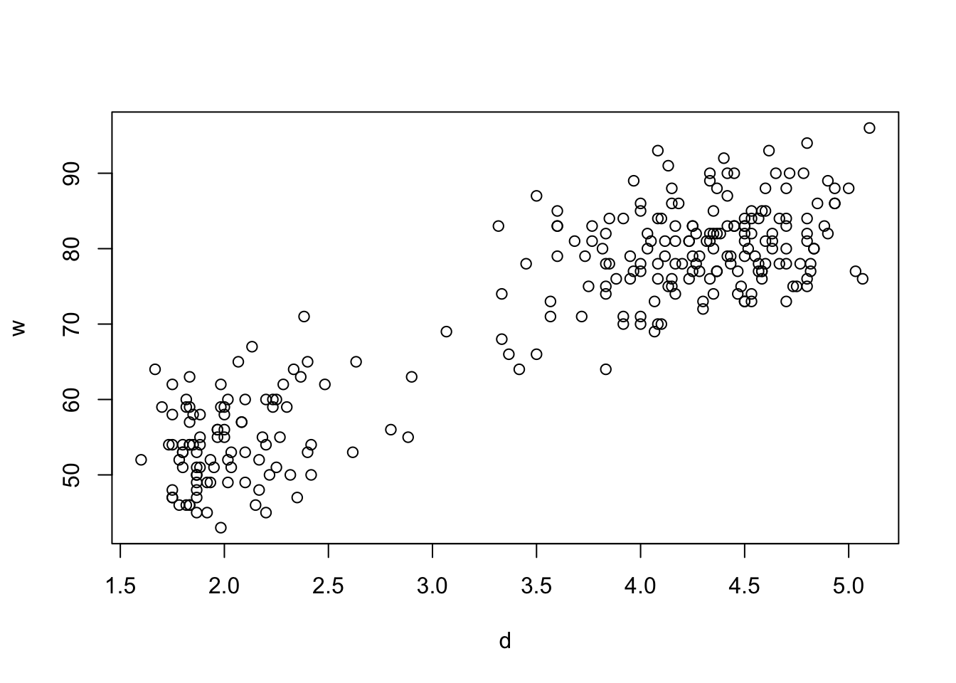
The model we’re interested in fitting to these data is a simple linear relationship between the waiting times, \(w\), and the eruption durations, \(d\): \[ w = {\beta_0}+ \beta_1 d + \varepsilon.\]
- Read the techniques page on changing axis limits, and then redraw your scatterplot so the horizontal axis covers the interval [0, 5.5], and the vertical axis covers [0, 100].
- Try guessing at some coefficients of the best-fitting straight line model. Use the
ablinefunction to draw the lines on your plot. Save your best guess asguess.b0andguess.b1. - Have a couple of attempts, but don’t spend too long! We’ll see better ways to do this next.
As mentioned above, the OLS method minimizes the square of the residuals which are the difference between the vector of observations, \(w_i\), and the fitted values, \(\widehat{w}_i\). Before we move on, let’s compute this sum-of-squares of errors value using your best guess at the coefficients.
- Using your best guesses as \(\widehat{\beta}_0\) and \(\widehat{\beta}_1\), create a vector called
guess.whatcontaining the fitted values \(\widehat{w}_i=\widehat{\beta}_0+\widehat{\beta}_1 d_i\) for your regression line. - Create a vector
guess.residcontaining the residuals \(e_i=w_i -\widehat{w}_i\). - Calculate the sum of squares of your residuals, \(Q(\)
guess.b0,guess.b1\()\). Save the value asguess.Q- we’ll compare it to the least-squares fit later.
3 Fitting the regression model
3.1 Direct calculation
We have access to all of the data and we know the formulae for the least squares estimates of the coefficients, so we should be able to calculate the best-fitting values directly
- First, calculate the regression summary statistics: use
meanto find \(\bar{w}\) and \(\bar{d}\) and save them aswbaranddbar. - Use the sample means with the original values of \(d\) and \(w\) to calculate \(S_{dd}\) and \(S_{dw}\) and store them as
sddandsdw. Hint: thesumfunction will be useful. - Use these summaries with the formulae in Section 1 to calculate the least-squares estimates \(\widehat{\beta}_0\), \(\widehat{\beta}_1\) and save them as
beta0hatandbeta1hat. - How do the least-squares estimates of the parameters compare to your guesses?
- Use the
ablinefunction to add the least-squares regression as an additional line to your plot. Use colour (thecolargument) to distinguish it from your previous guesses.
3.2 Linear regression with lm
It would be rather tiresome to have to do the calculations explicitly for every regression problem, and so R provides the lm function to compute the least-squares linear regression for us, and it returns an object which summarises all aspects of the regression fit.
In R, We can fit linear models by the method of least squares using the function lm. Suppose our response variable is \(Y\), and we have a predictor variable \(X\), with observations stored in R vectors y and x respectively. To fit \(y\) as a linear function of \(x\), we use the following lm command:
model <- lm(y ~ x)
Alternatively, if we have a data frame called dataset with variables in columns a and b then we could fit the linear regression of a on b without having to extract the columns into vectors by specifying the data argument
model <- lm(a ~ b, data=dataset)
The ~ (tilde) symbol in this expression should be read as “is modelled as”. Note that R always automatically include a constant term, so we only need to specify the \(X\) and \(Y\) variables.
We can inspect the fitted regression object returned from lm to get a simple summary of the estimated model parameters. To do this, simply evaluate the variable which contains the information returned from lm:
model
For more information, see Linear regression.
- Use
lmto fit waiting timeswas a linear function of eruption durationsd. - Save the result of the regression function to
model. - Inspect the value of
modelto find the fitted least-squares coefficients. Check the values match those you computed in the previous exercise.
R also has a number of functions that, when applied to the results of a linear regression, will return key quantities such as residuals and fitted values.
coef(model)andcoefficicents(model)– returns the estimated model coefficients as a vector \((\widehat{\beta}_0,\widehat{\beta}_1)\)fitted(model)andfitted.values(model)– returns the vector of fitted values, \(\widehat{y}_i=\widehat{\beta}_0+\widehat{\beta}_1 x_i\)resid(model)andresiduals(model)– returns the vector of residual values, \(e_i=y_i-\widehat{y}\)
For more information, see the R help page.
- Use the
coeffunction to extract the coefficients of the fitted linear regression model as a vector. Check the values agree with those obtained by direct calculation. - Extract the vector of residuals from
model, and use this to compute the sum of squares of the residuals aslsq.Q. - Compare
lsq.Qtoguess.Q- was your best guess close to the minimum of the least-squares error function?
3.3 The regression summary
We can easily extract and inspect the coefficients and residuals of the linear model, but to obtain a more complete statistical summary of the model we use the summary function.:
summary(model)
There is a lot of information in this output, but the key quantities to focus on are:
- Residuals: simple summary statistics of the residuals from the regression.
- Coefficients: a table of information about the fitted coefficients. Its columns are:
- The label of the fitted coefficient: The first will usually be
(Intercept), and subsequent rows will be named after the other predictor variables in the model. - The
Estimatecolumn gives the least squares estimates of the coefficients. - The
Std. Errorcolumn gives the corresponding standard error for each coefficient. - The
t valuecolumn contains the \(t\) test statistics. - The
Pr(>|t|)column is then the \(p\)-value associated with each test, where a low p-value indicates that we have evidence to reject the null hypothesis.
- The label of the fitted coefficient: The first will usually be
- Residual standard error: This gives \({s_e}\) the square root of the unbiased estimate of the residual variance.
- Multiple R-Squared: This is the \(R^2\) value defined in lectures as the squared correlation coefficient and is a measure of goodness of fit.
We can also use the summary to access the individual elements of the regression summary output. If we save the results of a call to the summary function of a lm object as summ:
summ$residuals– extracts the regression residuals asresidabovesumm$coefficients– returns the \(p \times 4\) coefficient summary table with columns for the estimated coefficient, its standard error, t-statistic and corresponding (two-sided) p-value.summ$sigma– extracts the regression standard errorsumm$r.squared– returns the regression \(R^2\)
- Apply the
summaryfunction tomodelto produce the regression summary for our example. Make sure you are able to locate:
- The coefficient estimates, and their standard errors,
- The residual standard error, \({s_e}^2\);
- The regression \(R^2\).
- Extract the regression standard error from the regression summary, and save it as
se. (We’ll need this later!) - What do the entries in the
t valuecolumn correspond to? What significance test (and what hypotheses) do these statistics correspond to? - Are the coefficients significant or not? What does this suggest about the regression?
- What is the \({R^2}\) value for the regression and what is its interpretation? Can you extract its numerical value from the output as a new variable?
4 Inference on the coefficicents
Given a fitted regression model, we can perform various hypothesis tests and construct confidence intervals to perform the usual kinds of statistical inference. To do this, we require the Normality assumption to hold for our inference to be valid.
Theory tells us that the standard errors for the parameter estimates are defined as \[ s_{\widehat{\beta}_0} = s_e \sqrt{\frac{1}{n}+\frac{\bar{x}^2}{S_{xx}}}, ~~~~~~~~~~~~~~~~~~~~ s_{\widehat{\beta}_1} = \frac{s_e}{\sqrt{S_{xx}}}, \] where \(s_{\widehat{\beta}_0}\) and \(s_{\widehat{\beta}_1}\) are unbiased estimates for \(\sigma_{\widehat{\beta}_0}\) and \(\sigma_{\widehat{\beta}_0}\), the variances of \(\widehat{\beta}_0\) and \(\widehat{\beta}_1\).
Given these standard errors and the assumption of normality, we can say for coefficient \(\beta_i\), \(i=0,1\) that: \[ \frac{\widehat{\beta}_i - \beta_i}{s_{\widehat{\beta}_i}} \sim \mathcal{t}_{{n-2}}, \] and hence an \(\alpha\) level confidence interval for \(\beta_i\) can be written as \[ \widehat{\beta}_i \pm t^*_{n-2,\alpha/2} ~ s_{\widehat{\beta}_i}. \]
- Consider the regression slope. Use the regression summary to extract the standard error of \(\widehat{\beta}_1\). Assign its value to the variable
se.beta1. - Compute the test statistic defined above using
beta1hatandse.beta1for a test under the null hypothesis \(H_0: \beta_1=0\). Does it agree with the summary output from R? - Use the
ptfunction to find the probability of observing a test statistic as extreme as this. - Referring to your \(t\)-test statistic and the
t values in the regression summary, what do you conclude about the importance of the regression coefficients? - Find a 95% confidence interval for the slope \(\beta_1\). You’ll need the Use the
qtfunction to find the critical value of the \(t\)-distribution. - Does this interval contain your best guess for \(\beta_1\)?
5 Estimation and prediction
Suppose now that we are interested in some new point \(X=x^*\), and at this point we want to predict: (a) the location of the regression line, and (b) the value of \(Y\).
In the first problem, we are interested in the value \(\mu^*=\beta_0+\beta_1 x^*\), i.e. the location of the regression line, at some new point \(X=x^*\).
In the second problem, we are interested in the value of \(Y^*=\beta_0+\beta_1 x^*+\varepsilon\), i.e. the actual observation value, at some new \(X=x^*\).
The difference between the two is that the first simply concerns the location of the regression line, whereas the inference for the new observation \(Y^*\) concerns both the position of the regression line and the regression error about that point.
Theory tells us that a \(100(1-\alpha)\%\) confidence interval for \(\mu^*\), the location of the regression line at \(X=x^*\), is
\[ (\widehat{\beta}_0 + \widehat{\beta}_1 x^*) \pm t^*_{n-2,\alpha/2} \times {s_e} \sqrt{\frac{1}{n} + \frac{(x^*-\bar{x})^2}{S_{xx}}} \]
Similarly, a \(100(1-\alpha)\%\) prediction interval for the location of the observation \(Y^*\) at \(X=x^*\) is
\[ (\widehat{\beta}_0 + \widehat{\beta}_1 x^*) \pm t^*_{n-2,\alpha/2} \times {s_e} \sqrt{1 + \frac{1}{n} + \frac{(x^*-\bar{x})^2}{S_{xx}}} \]
- Using the formulae above and the variables you have defined from previous questions, find a 95% confidence interval for the estimated waiting time \(\widehat{W}\) when the eruption duration is 3 minutes.
- Repeat the calculation to compute a 95% prediction interval for the actual waiting time, \(W\).
- Compare the two intervals.
6 Further exercises
If you finish the exercises above, have a look at some of these additional problems.