Practical 1-5: Hypothesis testing
Today we look at the properties of a hypothesis test for the fairness of a die. We simulate 120 rolls of a die and use our data to compare two competing hypotheses: one in which the die is fair, and the other in which the die has a specific bias towards 6. In particular, we will investigate the properties of the significance and the power of a hypothesis test.
- Download the R Script - Right click, and Save As
- You will need the following skills from previous practicals:
- Basic R skills with arithmetic, functions, etc
- Manipulating and creating vectors:
seq - Summarising data:
sum - Repeating calculations over a vector using
sapply - Plotting a scatterplot with
plot, and a histogram withhist
- New R techniques:
- Logical conditions and logical vectors, the
whichfunction - Subsetting elements of a vector using
[]
- Logical conditions and logical vectors, the
1 A simple hypothesis test
We will roll a die 120 times, and denote the number of times a 6 is rolled as \(X\). Let \(p\) be the probability of rolling a 6, with each roll of the die independent of the other rolls. We will use \(X\) to evaluate two competing hypotheses:
- Null Hypothesis \(H_0: p = \frac{1}{6}\)
- Alternative Hypothesis: \(H_1 : p = \frac{1}{6} + 0.02\)
That is, under the null hypothesis, the probability of rolling 6 agrees with that from a fair die, and the alternative hypothesis corresponds to a die biased towards 6.
We will define our test in terms of \(X\), the number of 6s rolled, and the goal will be to find a ‘good’ critical value \(x^*\) of \(X\), such that, if \(X \geq x^*\), we reject \(H_0\) in favour of \(H_1\). We will look at what ‘good’ means in terms of significance level and power of the test and will investigate the sort of experiment size required to get a good value of both as well as the behaviour of power as the bias changes.
2 Significance level
The significance level of a test, \(\alpha\), for a simple null hypothesis is the probability of rejecting \(H_0\) when \(H_0\) is true. For any chosen \(x^*\), the significance level of this test is \(\mathbb{P}[X \geq x^*]\), given \(H_0\).
Since the distribution for \(X\), the number of 6s rolled, is binomial with probability \(p\), we can use the binomial distribution to find \(\mathbb{P}[X \geq x]\) for any given value of \(x\). We can use R’s built-in binomial probability function to find the significance level for any particular \(x^*\).
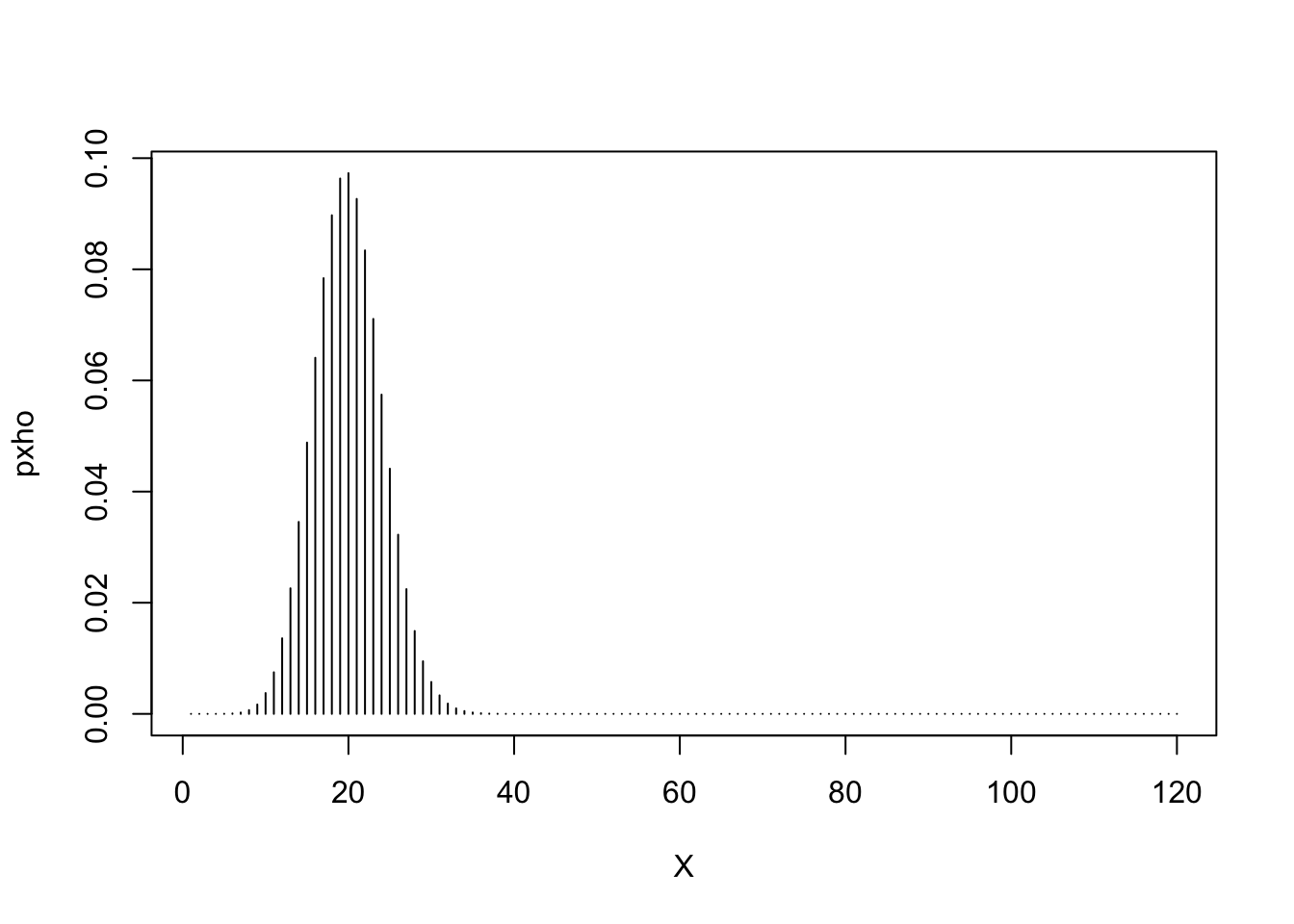
- First, create a vector of all of the possible numbers of 6’s that could be rolled, in this case the integers from 0 to 120. (Hint: use the
seqfunction or the:operator). Save this toX. - Next, calculate the probability of each outcome \(X\) under \(H_0\) by evaluating using the binomial probability mass function with \(n=120\) and \(p=\frac{1}{6}\) via the following command:
pxho <- dbinom(X, size=120, p=1/6) - Use
plotto draw a plot of \(X\) horizontally against the corresponding probability value vertically. Use the optional argumenttype='h'to draw a vertical line graph.
A logical vector is a vector that only contains the logical values of TRUE and FALSE. In R, true values are designated with TRUE, and false values with FALSE.
We will rarely construct these vectors directly, logical vectors are created by using comparison operators like < (less than), == (equals to), and != (not equal to) with numerical vectors.
==equal to!=not equal to<less than- `<= less than or equal to
>greater than>=greater than or equal to
For example
values <- 1:10
values > 5
## [1] FALSE FALSE FALSE FALSE FALSE TRUE TRUE TRUE TRUE TRUE
values ==4
## [1] FALSE FALSE FALSE TRUE FALSE FALSE FALSE FALSE FALSE FALSE
To extract a single value or subset of values from a vector, we use the syntax: a[index] where a is the vector, and index is a vector of index values.
values <- c(28, 67, 90, 23, 35, 16, 31, 69, 76, 83)
values[1]
## [1] 28
If we want multiple values from the vector, we can supply a vector of indices:
values[5:8]
## [1] 35 16 31 69
values[c(1,3,9)]
## [1] 28 90 76
We can also combine this idea of indexing with the idea of logical vectors introduced above. For instance, to extract only the values greater than 50:
values[values>50]
## [1] 67 90 69 76 83
Suppose we wanted to set the critical value \(x^*\) for our test to be \(X=20\), and we would reject the null hypothesis if we observed more 6s. This corresponds to the expected number of 6s in 120 rolls of the dice, and so we would reject if we observed more 6s than were expected.
- Create a logical vector of
TRUEandFALSEvalues corresponding to the statement \(X\geq 20\) - Hence, use the subsetting technique to select the entries of
pxhofor every \(X\geq 20\). - Add all of these selected values together using
sum
## [1] 0.5379619What we have just calculated is the significance level for a test which rejects \(H_0\) for \(X\geq 20\). Clearly, the significance value is quite high - and rather higher than the usual 5% or 1% values we’re used to. However, we can always raise the value of \(x^*\) which will lower the significance probability.
- Use
sapplyand a custom function which uses the code written above, evaluate the significance level for all 121 values of \(X\) in the vectorX. - Save your results to a vector called
alpha.
Given a logical vector, we may be interested in finding the indices of the vector which are TRUE. To do this we apply the which function:
which(values>50)
## [1] 2 3 8 9 10
which((1:12)%%2 == 0) # which of the integers 1 to 12 are even?
## [1] 2 4 6 8 10 12
Perhaps the most popular choice of significance level is 0.05. We can use the which function to find out which values of alpha are less than or equal to 0.05 by typing
which(alpha <= 0.05)
TRUE. The first value returned therefore corresponds to the index of the smallest value of \(x^*\) and the highest significance level which is acceptable.
- Evaluate
which(alpha <=0.05) - What is the index of the first value which satisfies this condition?
- Use subsetting to extract the corresponding elements of
Xandalphato find the values of \(x^*\) and \(\alpha\) for this approximate 5% test.
3 Power
For simple hypotheses, the power of a test is the probability of rejecting \(H_0\) when \(H_1\) is true. To work out the power of a test for a given significance level, we first select \(x^*\) appropriate to the chosen significance level and then compute \(\mathbb{P}[X >= x^*~|~H_1]\), the probability under \(H_1\) that we fall in the rejection region for our test and thus reject \(H_0\).
- Using the value of \(p\) specified in the alternative hypothesis, evaluate the probability of every outcome \(X\) under \(H_1\) using the binomial probability mass function.
- Use
sapplyto compute a vector of power values in the same way we computed the vector of significances. Call this vectorpowers.
If you have done this correctly, you should find that the power for \(x^* = 28\) is 0.1177323 which you can verify by returning the value of powers[29].
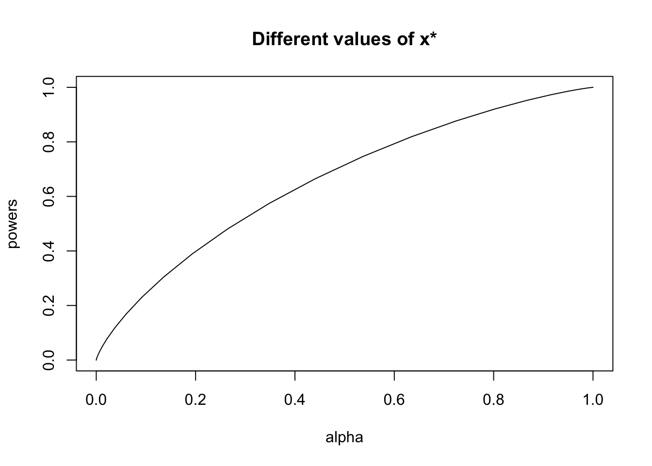
So, the price we have paid for having such a low probability of rejecting \(H_0\) when it is true (i.e. such a low significance level) is a low probability of rejecting \(H_0\) when \(H_1\) is true (i.e. a low power). We can see that there is a tradeoff between significance and power by plotting the two against each other.
- Use
plotto plot the significance values (alpha) horizontally against the power values (powers) vertically. Usetype='l'to join the values with lines.
For a given significance level, as we increase the sample size we will also increase the power of the test since extra data will provide more evidence for the test. There are two interesting questions raised by this initial exploration:
- how large does the sample size have to be to get a large power with a low significance, and
- how does the power change as the alternative hypothesis changes.
We look at the second question first.
3.1 The Power Function
Remembering that the significance level depends only on the null hypothesis, we can always choose \(x^* = 28\) to get a significance of less than 0.05. However, as we change the alternative hypothesis, the power of this test will change. The more extreme our alternative in comparison to the null hypothesis, the easier it should be to detect a difference between them and decide whether to reject or not.
We can look at what the power will be for all possible alternative hypotheses, by computing the power function. Suppose our alternative hypothesis is now
\(H_1 : p=\frac{1}{6} + a,~~~ \text{for}~ a\in \left( 0,\frac{5}{6}\right].\)
- Write a function called
powerFun, with argumenta, that computes the power of the hypothesis test for our critical value of \(x^*=28\), i.e. a significance level of 0.037.
- Create a sequence of 100 possible values for \(p\) under the alternative hypothesis. Hint: create a
sequencefrom0, toto5/6, and oflength100. Save this vector asp1vals. - Use
sapplyto apply your power function to every value inp1vals. Call the resulttPowers. - Plot
tPowersagainstp1valsas a line. Interpret the curve you see.
3.2 Variable Sample Size
We have seen how the power of the test changes as the bias in the alternative hypothesis changes. The other important question is how big a sample size is required to get a large power for the same significance.
Suppose we use our original hypotheses \(H_0\) and \(H_1\). We are now going to combine all of the steps taken in the previous sections in order to compute the power for different sample sizes.
- Write a function that takes
n, the number of die rolls, as an argument, and that finds the smallest \(x^*\) such that the significance level is not greater than 0.05, then uses that \(x^*\) to compute the power of the test with respect to the null hypothesis \(H_1\). Call this functionpowerFun2. - Hint: First, for given \(n\) you must calculate \(x^*\) using the null hypothesis as we did in Exercise 2.3. Then, you must compute the power for this value of \(x^*\) as we did in Excercise 2.4.
- For a range of sample sizes \(n\) from \(1\) up to \(250\), evaluate the power function and save the results as
power_vec. - Plot the power values
power_vecagainst the sample sizes \(n\). - Explain why powerFun2 generally increases with n.
3.3 Further exercises
The remaining exercises will require some careful thought and fair bit of R to answer. Attempt them if you have time:- By trial and error, find the smallest
nsuch that the significance level is not greater than 0.05 and the power is \(\geq\) 0.9. Call this valuenstar. Warning: Don’t try values of n bigger than around 5000 as these could take a long time to compute.
- For
n = nstarcalculate \(x^*\) using the first few lines of your function.
- Generate
nstarrolls from the die biased in the way described under \(H_1\). Count the number of 6s in the experiment.
- Based on the results of your simulation, would you reject \(H_0\)?
- Suppose the class has 20 people in it. If everyone completes the practical, how many would you expect to reject H0 based on their own simulations and this test?