$$ \def\ab{\boldsymbol{a}} \def\bb{\boldsymbol{b}} \def\cb{\boldsymbol{c}} \def\db{\boldsymbol{d}} \def\eb{\boldsymbol{e}} \def\fb{\boldsymbol{f}} \def\gb{\boldsymbol{g}} \def\hb{\boldsymbol{h}} \def\kb{\boldsymbol{k}} \def\nb{\boldsymbol{n}} \def\pb{\boldsymbol{p}} \def\qb{\boldsymbol{q}} \def\rb{\boldsymbol{r}} \def\tb{\boldsymbol{t}} \def\ub{\boldsymbol{u}} \def\vb{\boldsymbol{v}} \def\xb{\boldsymbol{x}} \def\yb{\boldsymbol{y}} \def\zb{\boldsymbol{z}} \def\Ab{\boldsymbol{A}} \def\Bb{\boldsymbol{B}} \def\Eb{\boldsymbol{E}} \def\Fb{\boldsymbol{F}} \def\Jb{\boldsymbol{J}} \def\Ub{\boldsymbol{U}} \def\xib{\boldsymbol{\xi}} \def\evx{\boldsymbol{e}_x} \def\evy{\boldsymbol{e}_y} \def\evz{\boldsymbol{e}_z} \def\evr{\boldsymbol{e}_r} \def\evt{\boldsymbol{e}_\theta} \def\evp{\boldsymbol{e}_r} \def\evf{\boldsymbol{e}_\phi} \def\evb{\boldsymbol{e}_\parallel} \def\omb{\boldsymbol{\omega}} \def\dA{\;\mathrm{d}\Ab} \def\dS{\;\mathrm{d}\boldsymbol{S}} \def\dV{\;\mathrm{d}V} \def\dl{\mathrm{d}\boldsymbol{l}} \def\bfzero{\boldsymbol{0}} \def\Rey{\mathrm{Re}} \def\Real{\mathbb{R}} \def\grad{\boldsymbol\nabla} \newcommand{\dds}[1]{\frac{\mathrm{d}{#1}}{\mathrm{d}s}} \newcommand{\ddy}[2]{\frac{\partial{#1}}{\partial{#2}}} \newcommand{\ddt}[1]{\frac{\mathrm{d}{#1}}{\mathrm{d}t}} \newcommand{\DDt}[1]{\frac{\mathrm{D}{#1}}{\mathrm{D}t}} $$
Magnetic helicity
I’ve always been intrigued by magnetic helicity as a global invariant of ideal MHD with a somewhat mysterious, gauge dependent character. I have made original contributions to both our theoretical understanding of helicity and its practical application and interpretation in solar physics.
Example. This video shows the build up of magnetic helicity in the solar corona over 60 days by surface shearing if we assume no new flux emergence [1]. The simulation uses the magneto-frictional model, with field lines are coloured by their field line helicity (red positive/blue negative), which integrates to give the global helicity.
Introduction
Writing \(\Bb=\nabla\times\textcolor{blue}{\Ab}\) allows us to uncurl the ideal-MHD induction equation: \[ \ddy{\Bb}{t} = \nabla\times(\ub\times\Bb) \quad \implies \ddy{\textcolor{blue}\Ab}{t} = \ub\times\Bb + \textcolor{blue}{\grad\phi}. \] It then follows that \[ \ddy{}{t}(\textcolor{blue}{\Ab}\cdot\Bb) = \grad\cdot\Big(\textcolor{blue}{\phi}\Bb + (\textcolor{blue}{\Ab}\cdot\ub)\Bb - (\textcolor{blue}{\Ab}\cdot\Bb)\ub\Big), \] so for a volume \(V\), the magnetic helicity \[ h(V) = \int_V\textcolor{blue}{\Ab}\cdot\Bb\,dV \] is conserved provided its flux vanishes on the boundary \(\partial V\).
Two broad challenges have motivated much of my work on magnetic helicity:
Gauge dependence. The choice of \(\textcolor{blue}{\Ab}\) is not unique, and under a gauge transformation \(\textcolor{blue}{\Ab'}= \textcolor{blue}{\Ab} + \textcolor{red}{\grad\chi}\), the magnetic helicity changes to \[ h'(V) = h(V) + \oint_{\partial V}\textcolor{red}{\chi}\Bb\cdot\hat{\nb}\,dS. \] For a magnetically-closed domain, this vanishes since \(\Bb\cdot\hat{\nb}=0\) on \(\partial V\), so \(h(V)\) is gauge-invariant. But for magnetically-open domains like the solar atmosphere, it does not. In this case, the value (and physical meaning) of \(h(V)\) depends on the gauge. Choosing a good one has been one of my main aims.
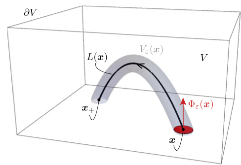
Decomposition. The standard way to avoid the gauge dependence problem is to use the Berger-Field relative helicity [2] instead of \(h(V)\). But this is not additive when \(V\) is decomposed into multiple sub-domains [3]. This is a problem in applications such as global coronal models where you want to know where the helicity is stored – e.g. to predict where eruptions might occur – or when your field contains helicity of both signs. For special decompositions, e.g. by concentric spheres or parallel planes, additivity holds between these regions. But a more general and flexible solution is to use field line helicity (FLH) – see our review chapter [4] or preprint.
Selected papers
[5] – Chris Prior and I showed how to give a physical/topological interpretation to magnetic helicity for magnetic fields stretching between two planes, when \(\Ab\) is in what we dubbed the winding gauge. Recently our PhD student Daining Xiao showed how to extend this nice interpretation to both spherical shell [6] and doubly-periodic [7] domains.
[1] – this novel paper studied how FLH is distributed and evolves in my global magneto-frictional model of the solar corona, as in the movie above. Note: the units in the figures were messed up so we issued a corrigendum [8].
[9] – postdoc Chris Lowder used FLH to identify magnetic flux ropes in our coronal MF model, as well as estimate the amount of flux and helicity they contain over the solar cycle.
[10] – the premise of this paper is how to define a FLH which integrates to give the Berger-Field relative helicity for a Cartesian box. See our book chapter [4] for more about the context. Our “relative FLH” requires a choice for the gauge of the reference \(\Ab\) on the boundary, and we proposed to use a minimal gauge for this.
[11] – with Gareth Hawkes (a PhD student at Exeter), we studied the (relative) helicity flux into the solar atmosphere using a data-driven surface flux transport model.
[12] – this paper addressed the problem in global coronal models that the Berger-Field relative helicity is a signed quantity, by defining an unsigned helicity based on FLH. An interesting consequence is that potential fields – which by definition have vanishing relative helicity – can have non-zero unsigned helicity. In a potential field, it’s dominated by “linkage” between active regions and the overlying field, and captures the helicity (and therefore energy) imparted purely by complexity of the surface magnetic configuration. I used unsigned helicity to analyse non-potential fields in [13].
See the magnetic braids page for applications of FLH to these, including our findings that it uniquely classifies their magnetic topology, and that it is dominantly redistributed rather than dissipated during turbulent relaxation.
Software
flhtools – Python+Fortran code for working with field-line helicity (and relative helicity) in a Cartesian box. This originally accompanied the paper [10].