R Techniques 10: Statistical methods

1 Statistical methods

1.1 Statistical tests in the stats package

1.1.1 \(t\) tests

The t.test function produces a variety of t-tests. Unlike most statistical packages, the default assumes unequal variance of the two samples, however we can override this with the var.equal argument.

# independent 2-sample t-test assuming equal variances and a pooled variance estimate
t.test(x,y,var.equal=TRUE)

# independent 2-sample t-test unequal variance and the Welsh df modification.
t.test(x,y)
t.test(x,y,var.equal=FALSE)

You can use the alternative="less" or alternative="greater" options to specify a one-sided test.

A paired-sample \(t\)-test is obtained from the same function by specifying paired=TRUE and ensuring both samples are the same size:

# paired t-test
t.test(x,y,paired=TRUE) 

Finally, a one-sample \(t\)-test can be performed to test the population mean \(\mu\) of the sample against a specific value by supplying only a single sample and a value for mu:

# one sample t-test
t.test(y,mu=3) # Ho: mu=3

R Help: t.test

1.1.2 Nonparametric tests of group differences

The nonparametric tests for comparing two samples can be performed in much the same way, only this time we use the wilcox.test function.

# independent 2-group Mann-Whitney U Test
wilcox.test(y,x) # where y and x are numeric

# paired 2-group  Signed Rank Test 
wilcox.test(y1,y2,paired=TRUE) # where y1 and y2 are numeric

R Help: wilcox.test

1.2 Linear regression

1.2.1 Fitting linear models with lm

Linear models can be fitted by the method of least squares in R using the function lm. Suppose our response variable is \(y\), and we have a predictor variable \(x\) and we want to \(y\) as a linear function of \(x\), we can use lm to do this:

model <- lm(y ~ x)

Alternatively, if we have a data frame called dataset with columns a and b then we could fit the linear regression of a on b without having to extract the columns by using the data argument

model <- lm(a ~ b, data=dataset)

The function lm fits a linear model to data and we specify the model using a ‘formula’ where the response variable is on the left hand side separated by a ~ from the explanatory variable(s). The formula provides a flexible way to specify various different functional forms for the relationship. The data argument is used to tell R where to look for the variables used in the formula. Note: The ~ (tilde) symbol should be interpreted as ‘is modelled as’.

For example, consider the data below from a study in central Florida where 15 alligators were captured and two measurements were made on each of the alligators. The weight (in pounds) was recorded with the snout vent length (in inches – this is the distance between the back of the head to the end of the nose). The data were analysed the data on the log scale (natural logarithms), and the goal is to determine whether there is a linear relationship between the variables:

alligator = data.frame(
  lnLength = c(3.87, 3.61, 4.33, 3.43, 3.81, 3.83, 3.46, 3.76,
               3.50, 3.58, 4.19, 3.78, 3.71, 3.73, 3.78),
  lnWeight = c(4.87, 3.93, 6.46, 3.33, 4.38, 4.70, 3.50, 4.50,
               3.58, 3.64, 5.90, 4.43, 4.38, 4.42, 4.25)
)
model <- lm(lnWeight~lnLength,data=alligator)

Inspecting the fitted regression lm object shows us a summary of the estimated model parameters:

model

## 
## Call:
## lm(formula = lnWeight ~ lnLength, data = alligator)
## 
## Coefficients:
## (Intercept)     lnLength  
##      -8.476        3.431

We can also add a fitted regression line to a plot by simply passing the fitted model to abline:

plot(y=alligator$lnWeight, x=alligator$lnLength)
abline(model,col='red')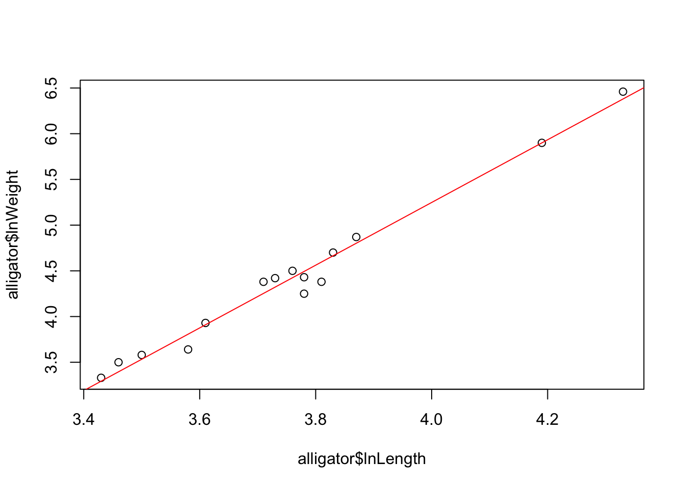

R Help: lm

1.2.2 The regression summary

The summary function in R is a multi-purpose function that can be used to describe an R object. It can be applied to vectors, matrices, data frames, linear models (lm objects), anova decompositions and many other R objects. Applying summary to our lm object via summary(model) will give a summary of many key elements of the regrssion:

summary(model)

## 
## Call:
## lm(formula = lnWeight ~ lnLength, data = alligator)
## 
## Residuals:
##      Min       1Q   Median       3Q      Max 
## -0.24348 -0.03186  0.03740  0.07727  0.12669 
## 
## Coefficients:
##             Estimate Std. Error t value Pr(>|t|)    
## (Intercept)  -8.4761     0.5007  -16.93 3.08e-10 ***
## lnLength      3.4311     0.1330   25.80 1.49e-12 ***
## ---
## Signif. codes:  0 '***' 0.001 '**' 0.01 '*' 0.05 '.' 0.1 ' ' 1
## 
## Residual standard error: 0.1229 on 13 degrees of freedom
## Multiple R-squared:  0.9808, Adjusted R-squared:  0.9794 
## F-statistic: 665.8 on 1 and 13 DF,  p-value: 1.495e-12

There is a lot of information in this output, but the key quantities are:

• Call: Printed here will be the formula of the regression model that was fitted.
• Residuals: This is a simple set of summary statistics of the residuals from the regression. Note that the mean of the residuals is always 0 and so is omitted.
• Coefficients: This is a table containing information about the fitted coefficients in the model and is the most useful part of the output. Its columns are:
  • The label of the fitted coefficient: The first will usually be (Intercept), indicating that the first row of the table contains information about the fitted intercept. Subsequent rows will be named after the other explanatory variables in the model forumula after the ~
  • The Estimate column gives the least squares estimates of the coefficients.
  • The Std. Error column gives the corresponding standard error for each coefficient.
  • The t value column contains the \(t\) test statistics for a test of the hypothesis \(H_0: \beta_i=0\) against \(H_0: \beta_i\neq 0\), for each coefficient \(\beta_i\).
  • The Pr(>|t|) column is then the \(p\)-value associated with that each test, where a low p-value indicates that we have evidence to reject the null hypothesis that the estimate is different from 0 (with the significance levels given by the number of stars).
• Residual standard error: This gives the square root of the unbiased estimate of the residual variance.
• Multiple R-Squared: For simple linear regression, this is the \(R^2\) value defined in lectures as the squared correlation coefficient and is a measure of goodness of fit (with values close to 1 indicating good fits to the data).
• Adjusted R-Squared: The adjusted R-Squared, \(\bar{R}^2\) is a penalised version of \(R^2\) which incorporates a penalty on the number of terms in the model to guard against unnecessarily overcomplicating the model. This is more useful when considering models with many predictors, and when comparing models with different numbers of predictors.
• F-statistic: and p-value: are the results of a hypothesis test that all coefficients other than the intercept are 0. This will be seen again in 3H.

R Help: summary

1.2.3 Extracting more detail

R also has a number of functions that, when applied to the results of a linear regression, will return key quantities such as residuals and fitted values.

• coef(model) and coefficicents(model) – returns the estimated model coefficients as a vector \((\widehat{\beta}_0,\widehat{\beta}_0)\)
• fitted(model) and fitted.values(model) – returns the vector of fitted values, \(\widehat{y}_i=\widehat{\beta}_0+\widehat{\beta}_0x_i\)
• resid(model) and residuals(model) – returns the vector of residual values, \(e_i=y_i-\widehat{y}\)
• confint(model, level=0.95) – CIs for model parameters
• predict(model, x, level=0.95) – predictions for the location of the SLR line, or for \(y\) at some new value x.

We can also extract the individual elements from the summary output from a regression analysis. Suppose we save the results of a call to the summary function of a lm object as summ. By using the $ we can extract even more valuable information from the components of the regression summary:

• summ$residuals – extracts the regression residuals as resid above
• summ$coefficients – returns the \(p \times 4\) coefficient summary table with columns for the estimated coefficient, its standard error, t-statistic and corresponding (two-sided) p-value.
• summ$sigma – the regression standard error
• summ$r.squared, summ$adj.r.squared – the regression \(R^2\) and adjusted \(R^2\) respectively
• summ$cov.unscaled – the \(p\times p\) (co)variance matrix for the least squares coefficients. The diagonal elements comprise the estimates of the variances for each of the \(p\) coefficients, and the off-diagonals give the estimated covariances between each pair of coefficients.

R Help: coef, fitted, resid, vcov, confint, predict,

1.2.4 More complex linear models

The following commands are for future reference and show the syntax of how to create linear models with multiple predictors, models with quadratic (or higher power) terms, and models with interaction terms.

## multiple regression involving 2 predictors
model1 <- lm(y ~ x1 + x2, data=myData) 
## quadratic regression on x1. Note each higher order term must be 
## enclosed within the I() function
model2 <- lm(y ~ x1 + I(x1^2), data=myData) 
## multiple regression with interaction
model3 <- lm(y ~ x1 + x2 + x1:x2, data=myData)
## more concise way of expressing model3
model3a <- lm(y ~ x1*x2, data=myData) 

R Help: lm, formula for more details on specifying a regression.