Practical 1-4: Bayesian analysis of Poisson data
In this practical we use R to investigate the conjugate Bayesian analysis for Poisson data. We will also investigate using the effects of the prior distribution on the posterior, and the situation where our sample size grows large.
- Download the R Script - right click, and Save As
- You will need the following skills from previous practicals:
- Creating vectors with
seq - Drawing a plot of a known function using
curve - Using additional graphical parameters to customise plots with colour
(
col), line type (lty), axis range (xlimandylim) etc - Adding simple straight lines to plots with
abline - Writing your own functions with
function
- Creating vectors with
- New R techniques:
- Using
plotto draw plots of general data, andlinesandpointto add additional data - Using R’s built-in functions to evaluate a standard pdf,
e.g.
dgammaanddnorm - Using the quantile functions, e.g.
qgamma, to produce exact credible intervals using standard distributions - Using
sapplyto evaluate a function with different arguments specified by the element of a vector
- Using
1 The Data
Our dataset concerns the number of volcanoes that erupted each year from 2000 to 2018, taken from here. The data are given in the table below, where each volcanic eruption is counted in the year that the eruption started. Volcanic eruptions are split into groups depending on the severity of the eruption, as measured on the logarithmically-scaled Volcanic Explosivity Index (VEI). For example, the 2010 eruption of Eyjafjallajökull in Iceland had a VEI of 4, whereas the eruption of Krakatoa in 1883 was VEI6.
The eruptions are loosely classified as Small (VEI\(\leq 2\)), Medium (\(2<\) VEI \(<4\)), and Large (VEI \(\geq 4\)).
| Year | 2000 | 2001 | 2002 | 2003 | 2004 | 2005 | 2006 | 2007 | 2008 | 2009 |
| Small | 30 | 25 | 30 | 32 | 29 | 29 | 34 | 29 | 25 | 28 |
| Medium | 6 | 6 | 5 | 5 | 8 | 4 | 3 | 3 | 7 | 2 |
| Large | 0 | 0 | 0 | 2 | 1 | 1 | 1 | 3 | 2 | 1 |
| Year | 2010 | 2011 | 2012 | 2013 | 2014 | 2015 | 2016 | 2017 | 2018 |
| Small | 39 | 30 | 40 | 40 | 41 | 26 | 37 | 30 | 34 |
| Medium | 6 | 6 | 4 | 7 | 7 | 5 | 4 | 6 | 4 |
| Large | 3 | 0 | 1 | 0 | 1 | 0 | 2 | 0 | 1 |
- Run the
Rcode below to input the data, and create a new data frame calledvolcano, with columnsYear,Small,Medium, andLarge.
volcano <- data.frame(Year = 2000:2018,
           Small = c(30, 25, 30, 32, 29, 29, 34, 29, 25, 28, 39, 30,
                     40, 40, 41, 26, 37, 30, 34),
           Medium = c(6, 6, 5, 5, 8, 4, 3, 3, 7, 2, 6, 6, 4, 7, 7,
                      5, 4, 6, 4),
           Large = c(0, 0, 0, 2, 1, 1, 1, 3, 2, 1, 3, 0, 1, 0, 1,
                     0, 2, 0, 1))
Plot, points, and lines
The plot function produces a scatterplot of its two
arguments. Suppose we have saved our \(x\) coordinates in a vector a,
and our \(y\) coordinates in a vector
b, then to draw a scatterplot of \((x,y)\) we type
plot(x=a, y=b)
If the argument labels x and y are not
supplied, R will assume the first argument is x
and the second is y. If only one vector of data is
supplied, this will be taken as the \(y\) value and will be plotted against the
integers 1:length(y), i.e. in the sequence in which they
appear in the data.
All of the standard plot functions can be customised by passing additional arguments to the function. For instance, we can add a plot title and axis labels by supplying optional arguments:
type- determines the type of plot to draw. Possible types are:- “p” for points
- “l” for lines
- “b” for both (points connected by lines)
- “h” for histogram-like vertical lines
- “s” for step lines
xlab,ylab- provides a label for the horizontal and vertical axesxlim,ylim- allows for specification of a minimum and maximum value of the corresponding axis limits, e.g.xlim=c(0,10)will set the horizontal axis limits to be \([0,10]\).col- can be specified to use colour for drawing
For example,
plot(x=-10:10,y=sin((-10:10)/(2*pi)), type="b", xlab='A', ylim=c(-1.5,1))
Note: Once a plot has been drawn, it is not possible to
erase any features from it - we can only add extra lines or points to
it. So, if you make a mistake drawing your plot then you’ll need to
start over with a fresh one by calling plot again.
After creating a plot, we can add additional
points to the plot by calling the points function which
draws additional points at the specified x and
y values. Similarly, the lines function will
draw connected lines between its x and y
arguments.
plotthe number ofSmalleruptions against the year using a vertical axis range (ylim) of \([0,50]\).- Experiment with the plot
types to see how the different plots represent the data. - Redraw the data as a
lineplot, and addlinesof different colours to the same plot for the other two groups of eruptions. - Do you see any apparent relationship between time and number of eruptions?
- Now plot the
histogram of the number ofMediumeruptions - does it look like it could follow a Poisson distribution? How else could you quickly assess this?
2 Conjugate analysis with the Gamma-Poisson model
2.1 The Theory
A Poisson distribution is often used to model the counts of random events occurring within a fixed period of time at some rate \(\lambda\). For such a random variable \(X\) where \(X\sim\text{Po}(\lambda)\) , a Bayesian analysis will require a prior distribution for the unknown Poisson parameter \(\lambda\). We have seen that the Gamma distribution provides a conjugate prior for this particular problem. Therefore, if our data \(X_1,\dots,X_n\) are \(\text{Po}(\lambda)\), and our prior distribution for \(\lambda\) is \(\text{Ga}(a,b)\). Then the posterior distribution for \(\lambda ~|~ X_1,\dots,X_n\) is given by: \[ \lambda ~|~ X_1,\dots,X_n \sim \text{Ga}(a+T, b+n), \] where \(T=\sum_{i=1}^n X_i= n\overline{X}\).
2.2 The prior
First, let’s use the Gamma distribution to identify an appropriate prior for our Poisson count data.
Standard density functions in R
R provides built-in functions to evaluate the PDF of
standard distributions. The density function for a Gamma distribution
\(\text{Ga}(a,b)\) is used as
follows
dgamma(x, shape=a, rate=b)
where x is the point (or vector of points) where we want
to evaluate the PDF, and a and b are the usual
Gamma parameter values.
- Create a vector containing a
sequence of 500 equally-spaced values over the interval \([0,10]\). Call thislambdavals. - Evaluate the \(\text{Ga}(1,1)\) pdf
at each of the values of \(\lambda\) in
lambdavalsusing the gamma PDFdgamma. - Make a
plotof the pdf against \(\lambda\) as a solid black line.
An expert vulcanologist believes that the unknown rate of
Medium eruptions, \(\lambda\), is such that a range of \([1,6]\) would be plausible.
You may need to use a pen and paper to do some maths to answer some of the following exercise!
- Interpret the expert’s given interval as corresponding to a statement of \(\mathbb{E}(\lambda) \pm 2\text{sd}(\lambda)\). Using this statement and the expert’s interval given above, find the value of the mean (\(\mathbb{E}(\lambda)\)) and variance (\(\mathbb{V}\text{ar}(\lambda)=\text{sd}(\lambda)^2\)) of the prior distribution for \(\lambda\).
- Equate the prior mean and variance you have just found to the theoretical values for the expectation (\(a/b\)) and variance (\(a/b^2\)) of a Gamma pdf. Solve these two equations to find the expert’s corresponding values of the parameters \(a\) and \(b\).
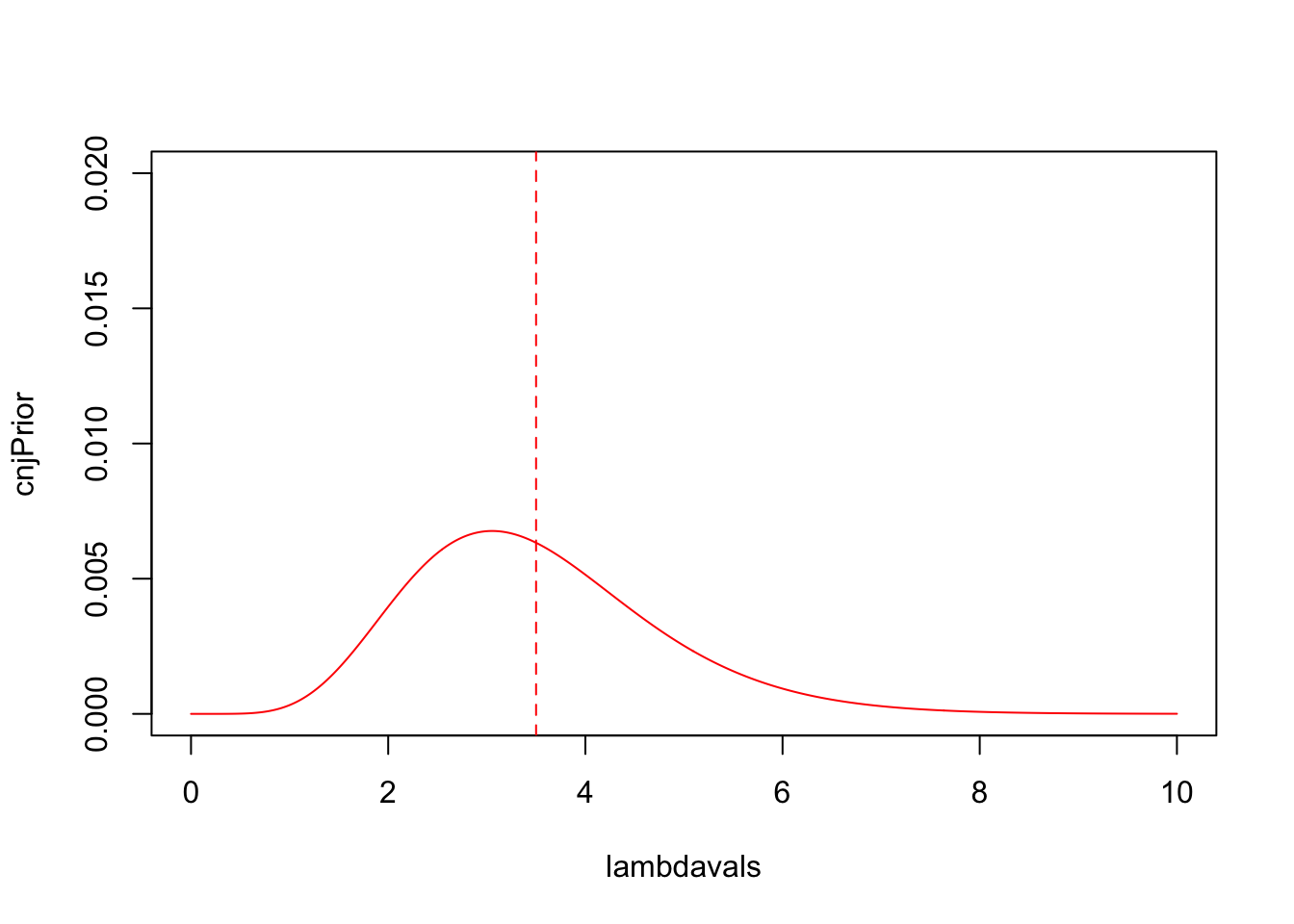
- Evaluate the expert’s prior pdf for \(\lambda\) at each of
lambdavals, and save it ascnjPrior. - For plotting purposes, we need to normalise the values of
cnjPriorso that they sum (integrate) to 1. Divide the values ofcnjPriorby thesumof the values incnjPrior, and replacecnjPriorby these normalised values. - Produce a fresh plot of the expert’s prior pdf for \(\lambda\) as a solid red curve. Ensure your vertical axis covers \([0,0.02]\).
- Add a vertical red and dashed line (
ablineusing thevargument) at the location of the prior expectation for \(\lambda\).
Quantiles of standard densities
In addition to built-in functions for PDFs of standard distributions,
R also provides the quantile function for a pdf.
The quantile function evaluates the inverse of the cumulative
distribution function, \(F_X^{-1}(u)\).
Given a probability value \(u\in[0,1]\), the quantile function returns
the value \(x\) of \(X\) for which \(P[X\leq x]=u\), and so the quantile
functions are particularly useful for finding critical values of
distributions and for finding exact credible intervals.
The quantile function for a Gamma density \(X\sim \text{Ga}(a,b)\) is used as follows
qgamma(alpha, shape=a, rate=b)
where alpha is the lower tail probability (or vector of
lower-tail probabilities) for which we want the corresponding value(s)
of \(X\), and a and
b are the usual Gamma parameter values.
- Use the
qgammafunction to find a 95% equal-tailed prior credible interval for \(\lambda\) using the expert’s prior distribution above. Hint: find the values of \(\lambda\) with lower and upper tail probabilities of \(2.5\%\). - How does this compare to the expert’s original interval?
2.3 The likelihood
The next ingredient in the Bayesian calculation requires us to capture the information contained in the data via the likelihood. In a Bayesian context, the likelihood is the conditional distribution of the data \(X_1,\dots, X_n\) given the parameter \(\lambda.\)
Let’s compute the likelihood given our data on Medium
volcanic eruptions, and add it to the plot.
- Write a function
poisLikethat computes the Poisson likelihood for the sample ofMediumvolcano eruptions. Your function should:- Take one argument
lambda - Compute the Poisson probability for each data point in
volcano$Mediumgiven the value oflambda. Hint: thedpoisfunction evaluates Poisson probabilities for a vector of valuesxand parameterlambda. Or you can use your own function from last time. - Combine the probabilities to find the likelihood of the entire
sample, and
returnit. - If your function is working correctly, you should agree with the output below.
- Take one argument
poisLike(5)## [1] 4.225604e-17Using sapply to repeat calculations over a
vector
We have seen previously that we can use the replicate to
repeatedly call a function with no arguments. For functions which do
take an argument, we often want to call that function at many different
values. To do this, we use sapply to apply a specified
function to every element of a vector as its argument, and then return a
vector formed from the results.
sapply(x, fun)
applies the function fun to every element of the vector
x it then returns a vector containing the values of
fun(x[1]), fun(x[2]), and so on. So, to
compute the square-root of the integers \(1\) to \(10\), we would write
sapply(1:10, FUN=sqrt)
or alternatively
which applies the square root function to each of the integers 1 to 10.
There are other variations of apply which work with
matrices and other data structures, and we will see those in later
practicals.
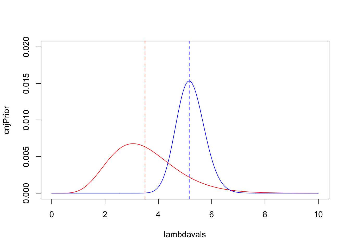
- Use
sapplyto evaluate the Poisson likelihood (poisLike) for each of the values of \(\lambda\) inlambdavals. Save this aslike. - Normalise
likeso that its values sum to \(1\). - Add the likelihood to your plot of the prior distribution as
connected blue
lines. - Add the maximum likelihood estimate of \(\lambda\) as a vertical dashed blue line.
- Your plot should look like the one below
2.4 The posterior
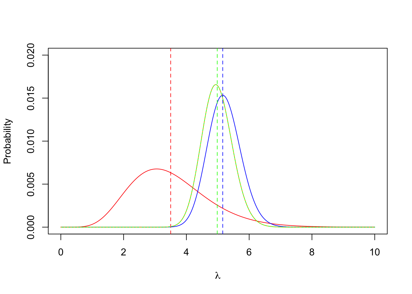
We can apply Bayes rule directly, given the prior and likelihood, and numerically compute the posterior density for all of the values of \(\lambda\).- Directly compute the posterior for \(\lambda\) by Bayes theorem, and save these
values as
postDirect. Normalise thepostDirectso that it sums to \(1\). Hint: \(\text{Posterior} \propto \text{Likelihood} \times \text{Prior}\). - Add the posterior to your plot as a solid green curve.
However, we also know that we’re using the conjugate Gamma prior with a Poisson likelihood, so our posterior distribution for \(\lambda\) will also be a Gamma with parameter values as above. Let’s verify that this is the case, and add the resulting density function to our plot.
- Now use conjugacy to evaluate the conjugate Gamma posterior
distribution.
- First find the posterior values of the Gamma parameters \(a\) and \(b\), save these as
aPostandbPost. - Now use
dgammawith the posterior parameter values to evaluate the posterior Gamma density at each oflambdavals. Save these values topostConjugateand normalise to sum to \(1\).
- First find the posterior values of the Gamma parameters \(a\) and \(b\), save these as
- Draw the conjugate posterior on your plot as a dashed
purplecurve. - What do you see? Do the results agree with each other? How has the prior changed?
- Add the posterior mean as a vertical green line.
- What do you notice about the relationship between the posterior mean, the prior mean, and the maximum likelihood estimate?
- Use the exact Gamma posterior to find a 95% posterior credible interval for \(\lambda\).
- Compare the posterior interval with the prior interval you found earlier. What has changed?
3 Further Exercises: Exploring the effects of prior choice and sample size
3.1 Changing the prior parameters
To investigate how sensitive our results are to our choices for \(a\) and \(b\) in the prior Gamma distribution, we’re going to want to repeat our previous calculations for different values of the prior parameters. To make this easier, let’s wrap those calculations and plots in a new function that finds and draws the Gamma posterior for a given prior and data set:
- Write a function called
gammaPoissonwhich:- Takes four arguments: the prior Gamma parameters
aandb, and the summary statisticsTandn. - Computes the \(\text{Ga}(a,b)\)
prior and the \(\text{Ga}(a+T,b+n)\)
posterior over the sequence of values in
lambdavals. - Plots the (normalised) prior and posterior Gamma distributions as coloured curves on one plot.
- Adds the MLE as a dashed vertical line.
- Takes four arguments: the prior Gamma parameters
- Check your function by evaluating it with the values of
a,b,T, andnwe used for theMediumvolcano data above.
- Investigate what happens as you change
aandb.- How does the shape of the prior change? What impact does this have on the posterior distribution?
- What happens for large values of
aandb? How does this affect your results?
3.2 Updating beliefs with large samples
In Lecture 26, we will see that show that as the sample size grows large, the posterior distribution tends towards a Normal distribution and the posterior distribution becomes progressively less affected by the choice of prior distribution.
Let’s expand our data with the records of volcanic eruptions for the
entire 20th century. As records are slightly incomplete, only the counts
of Large eruptions over this period can be considered
trustworthy. For the entire 100 years, a total of 64 Large
(VEI\(\geq 4\)) eruptions were
recorded
- Combine the 20th century data with the data from 2000-2018 and
compute new summary statistics for the
Largevolcanic eruptions from 1900-2018. Save these asTbigandNbig. - Use a prior of \(\lambda\sim\text{Ga}(2,2)\), and plot the posterior given the combined data. What happens to the posterior?
The large sample of data is clearly very informative for \(\lambda\), resulting in a posterior distribution that is concentrated over a small range of possible \(\lambda\) values. Let’s refocus our plot on that sub-interval:
- By modifying your Gamma-Poisson function, redraw the same plot to
zoom in on the interval \(\lambda\in[0.25,1.25]\). Hint: you’ll need
to set the
xlimargument toplot(or add it as an argument to your function). - What do you notice about the shape of the Gamma posterior distribution?
3.2.1 Theory: Limiting posterior distribution
If we suppose that \(X=(X_1,\dots,X_n)\) are an i.i.d. sample of size \(n\) from a distribution with pdf \(f(x~|~\theta)\) where \(X_i \perp X_j ~|~ \theta\) and \(f(x~|~\theta)\) is twice differentiable, then for \(n\) ‘large enough’ the posterior distribution for \(\theta ~|~ x\) is approximately \[ f(\theta ~|~ x) \approx \text{N}\left(\widehat{\theta}, \frac{1}{{I}\left(\widehat{\theta}\right)}\right), \] where \(\widehat{\theta}\) is the MLE of the parameter \(\theta\), and \(\text{I}(\widehat{\theta})\) is the observed Fisher information for a sample of size 1.
For a Poisson distribution, we have:
- \(\widehat{\lambda}=\frac{\sum_i x_i}{n}\)
- \(\mathcal{L}''(\lambda)=-\frac{\sum_i x_i}{\lambda^2}\).
- Using the results above, compute the mean and variance of the
limiting posterior distribution for the
Largevolcano eruption data. - Using
dnorm, evaluate the Normal approximation to the posterior pdf for \(\lambda\) overlambdavals. Normalise it again to sum to one, and add it to your plot using a thick dashed line. - Is the limiting normal distribution in agreement with the Gamma posterior? If it differs, how does it differ and to what extent?
- Do the values of the Gamma prior parameters \(a\) and \(b\) affect the quality of the approximation?