Topic 6 - Differential Equations

6.0 Introduction

An ordinary differential equation (ODE) is an equation connecting a function and some of its derivatives. These are extremely common across the sciences.

Example 6.1. $(1)\;$ Falling object:$\;$ The velocity $v(t)$ at time $t$ of a stone of mass $m$ falling under gravity satisfies the differential equation \[m\frac{dv}{dt}=mg-\lambda v^2\] where $\lambda$ is a constant measuring air resistance.

$(2)\;$ Radioactive Decay:$\;$ Radiation given out is proportional to the amount $y(t)$ of radioactive substance present at time $t$, i.e. \[\frac{dy}{dt}=-ky\] where $k$ is a positive constant determined by the half-life.

$(3)\;$ Electrical circuits:$\;$ Recall an RLC circuit is a combination of resistors, inductors and capacitors. A time-varying voltage source $V(t)$ is placed across a series circuit consisting of a resistor $R$, an inductor $L$ and a capacitor $C$ (all measured in suitable units).

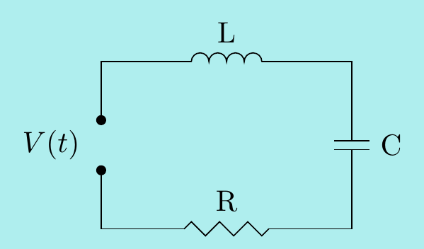
The current $I(t)$ at time $t$ in the circuit satisfies a differential equation: \[L\dfrac{d^2I}{dt^2}+R\dfrac{dI}{dt}+\dfrac{I}{C}=\dfrac{dV}{dt}\]

There are of course many more examples such as Newton’s law of cooling, forced oscillations of a damped spring, bending moments, missile pursuit, cables of a suspension bridge,… One can also consider systems of differential equations, linking multiple functions and their derivatives. For instance, the phugoid equations \[\frac{dv}{dt}=-\sin\theta-Rv^2,\qquad \frac{d\theta}{dt}=\frac{v^2-\cos\theta}{v}\] model the complicated behaviour of the velocity $v(t)$ and angle to the horizontal $\theta(t)$ of a paper airplane. We will look at some (much simpler!) systems at the end of the Topic.

It’s also possible to consider partial differential equations (PDEs) which involve partial derivatives. For instance, a vibrating string has a displacement $u(x,t)$ at position $x$ and time $t$ governed by the wave equation \[\dfrac{\partial^2 u}{\partial t^2}=c^2\dfrac{\partial^2 u}{\partial x^2}.\] PDEs are generally much harder to solve and we won’t consider them in this module.

General and particular solutions

We start by looking at a very easy ODE \[\frac{d^2y}{dx^2}=0.\] This is an ODE of order $2$. Generally, the order of an ODE is the order of the highest derivative that occurs in it.

Clearly $y=x$ is a solution, but it is not the only one. For example, $y=3x+1$ is also a solution. In fact, by integrating twice we see that the solutions are given by \[y=Ax+B\] for any real constants $A,B$. There are two constants here because we needed to integrate twice to solve the ODE. When solving an ODE of order $n$, we will get $n$ arbitrary constants in the general solution. Then, a particular solution is determined by $n$ conditions (often called initial conditions) in order to determine these constants. For instance, in the example above, $y=Ax+B$ is the general solution, and to find a particular solution, e.g. with initial conditions $y(0)=1$, $y'(0)=2$, we need to find $A,B$ such that \[\begin{align*} 1&=y(0)=A\times0+B \\ 2&=y'(0)=A. \end{align*}\] Hence $A=2,\ B=1$ and the required particular solution is $y=2x+1$.

Of course, the above ODE is very simple. Unfortunately, there is no one method for solving ODEs - this should be reminiscent of how there is no single method for calculating all integrals. Indeed, some can only be attacked by numerical methods. However, because they are so important and so common in the sciences, many special methods have been developed and we take the following general approach:

Classify the type and write the ODE in a standard form.
Apply a suitable method to find the general solution to the ODE.
If we want a particular solution, use the conditions to determine the arbitrary constants

A generic first order ODE can be written in the form: \[\frac{dy}{dx}=f(x,y)\] for some function $f(x,y)$. There isn’t even a general method to solve these, but in the next few sections, we’ll look at some special cases where suitable methods are available.

6.1 First order ODEs: Separable Equations

First order ODEs involve only first derivatives so the general solution will involve one arbitrary constant. A particular solution is then determined by a single condition.

The most basic type of differential equation is of the form \[\frac{dy}{dx}=f(x)\] for some function $f(x)$. To solve it, we just integrate to find \[y=\int f(x)\,dx.\] The integration constant is the arbitrary constant in this general solution. Notice this simplest type of ODE is at least as hard as integration!

We can generalise slightly to separable equations. These have the form: \[\frac{dy}{dx}=f(x)g(y)\] so the right-hand-side is a product of a function of $x$ and a function of $y$.

Method of solution.$\;$ We separate the variables $x$ and $y$ by cross-multiplying and then integrating: \[\int\frac{dy}{g(y)}=\int f(x)\,dx .\] Solving separable ODEs is thus only as hard as finding two integrals.

Example 6.2. Solve the separable equation $\;\;\dfrac{dy}{dx}=xe^{-x}e^y\;\;$ where $y(0)=0$.

We first separate the variables and write down two integrals: \[\int e^{-y}\,dy=\int xe^{-x}\,dx.\] Integrating both sides (using parts on the $x$ integral) gives \[-e^{-y}=-xe^{-x}+\int e^{-x}\,dx=-xe^{-x}-e^{-x}+A=-e^{-x}(x+1)+A.\] Both integrals get an integration constant but we can combine them into a single one on one side. Now rearranging gives the general solution for $y$ in terms of $x$. \[y=-\ln\left(e^{-x}(1+x)-A\right).\] We can finally obtain the value of $A$ from the condition: \[y(0)=0\quad\implies\quad -\ln\left(e^0(1+0)-A\right)=0 \quad\implies\quad A=0\] and the particular solution is $y=-\ln\left(e^{-x}(1+x)\right)=x-\ln(1+x)$.

Once one has a solution, it’s easy to check if it is correct: just substitute it back to the equation and see if it works.

It’s not always possible to rewrite the solution to give $y$ in terms of $x$.

Example 6.3. Solve the separable equation $\;\; \dfrac{dy}{dx}=(x^2-1)\dfrac{y}{y+1}$.

Separating and integrating gives \[\begin{align*} \int\frac{y+1}{y}\,dy=\int (x^2-1)\,dx \quad\implies\quad y+\ln|y|=\frac13x^3-x+A. \end{align*}\] There is no way to rewrite this as $y$ equals a function of $x$ so we just have to leave the general solution in this implicit form.

Example 6.4. Solve the separable equation $\;\;\dfrac{dy}{dx}=(1+x)\left(\dfrac{1+y^2}{2y}\right)\;\;$ where $y(0)=2$.

We just cross-multiply and integrate: \[\begin{align*} \int\frac{2y}{1+y^2}\,dy&=\int (1+x)\,dx \\ \implies \ln\left(1+y^2\right)&=x+x^2/2+A \\ \implies 1+y^2&=e^{x+x^2/2+A} \\ &=e^{x+x^2/2}e^A \\ &=Be^{x+x^2/2} \quad\text{where $B=e^A$} \\ \implies y&=\pm\sqrt{Be^{x+x^2/2}-1} \end{align*}\] This is the general solution and using the given initial condition, \[2=y(0)=\pm\sqrt{B-1}\quad \implies\quad B=5\] and the particular solution is $\;\;y=\pm\sqrt{5e^{x+x^2/2}-1}$. But wait: it seems there are two solutions? However, to obtain $y(0)=2$, we must only take the positive square root.

In the above examples, it was obvious the equation was separable. Sometimes we have to do a bit of work to get it in the correct form first.

Example 6.5. Solve the equation $\;\;2y\dfrac{dy}{dx}-x-y^2=1+xy^2$.

Rewrite this as \[\begin{align*} \frac{dy}{dx}&=\frac{1}{2y}\left(1+xy^2+x+y^2\right) \\ &=\frac{1}{2y}\left(1+x+\left(1+x\right)y^2\right) \\ &=\frac{1}{2y}\left(1+x\right)\left(1+y^2\right) =(1+x)\left(\frac{1+y^2}{2y}\right) \end{align*}\] This the now the same ODE as in the previous example.

6.2 First order ODEs: Homogeneous Equations

A homogeneous first order ODE has the form \[\frac{dy}{dx}=f\left(\frac{y}{x}\right).\]

Method of solution:$\;$ Make the substitution $u=\dfrac{y}{x}$. Applying the product rule to $y=ux$ gives \[\frac{dy}{dx}=u+\frac{du}{dx}x \] so the ODE becomes \[ u+\frac{du}{dx}x=f(u)\quad\implies\quad \frac{du}{dx}=\frac{1}{x}\left(f(u)-u\right)\] We have converted the equation into a separable ODE and can now apply the previous section to find $u$ and hence find $y=ux$.

Example 6.6. Find the general solution of $\;\;\dfrac{dy}{dx}=\left(\dfrac{y}{x}\right)^2+\dfrac{y}{x}+1$.

Put $y=ux$ so that $\dfrac{dy}{dx}=u+\dfrac{du}{dx}x$. Then the ODE becomes \[u+\frac{du}{dx}x=u^2+u+1 \quad\implies\quad \frac{du}{dx}=\frac{u^2+1}{x}. \] Solving this separable equation: \[\begin{align*} \int\frac{1}{u^2+1}\,du=\int\frac{1}{x}\,dx &\quad\implies\quad \arctan u=\ln |x|+A \\ &\quad\implies\quad u=\tan\left(\ln |x|+A\right). \end{align*}\] Hence the general solution is $\;\;y=xu=x\tan(\ln |x|+A)$.

Again, it is not always immediately obvious that an ODE is homogeneous so we might have to do a bit of work to get it in the right shape.

Example 6.7. Solve the equation $\;\;x^2\dfrac{dy}{dx}=y^2+xy+x^2$.

Simply dividing both sides by $x^2$ gives the same ODE in the previous example.

Remark. If we are given an ODE in the form $\dfrac{dy}{dx}=g(x,y)$, then we can generally tell if it is homogeneous by checking that \[g(\lambda x,\lambda y)=g(x,y)\quad\text{for all constants $\lambda$}.\] This says that $g(x,y)$ only depends on the ratio of $y$ and $x$ so can be written as $f(y/x)$.

6.3 First order ODEs: Linear Equations

A linear first order ODE has the form \[\frac{dy}{dx}+f(x)y=g(x).\] Method of solution:$\;$ We define a new function, called the integrating factor, by \[\displaystyle I(x)=\exp\left(\int f(x)\,dx\right).\]

By the chain rule, this satisfies $\dfrac{dI}{dx}=I(x)f(x)$. Now multiply both sides of the ODE by $I(x)$ to obtain

\[\begin{align*} I(x)\frac{dy}{dx}+I(x)f(x)y=I(x)g(x) &\quad\implies\quad I(x)\frac{dy}{dx}+\frac{dI}{dx}y=I(x)g(x) \\ &\quad\implies\quad \frac{d}{dx}\bigl(I(x)y\bigr)=I(x)g(x). \end{align*}\] We can now integrate both sides to get $\;\displaystyle I(x)y=\int I(x)g(x)\,dx+A$ and so we obtain the general solution \[y=\frac{1}{I(x)}\left(\int I(x)g(x)\,dx+A\right). \]

(Note: don’t learn this formula! Learn the method…)

Example 6.8. Solve the equation $\;e^{-x}\dfrac{dy}{dx}+2xe^{-x}y=2x+1$, where $y(0)=3$.

We first write it in the standard form $\;\dfrac{dy}{dx}+2xy=e^x\left(2x+1\right)$.

The integrating factor is $\;I(x)=\exp\left({\int 2x\,dx}\right)=e^{x^2}$.

Now multiply both sides of the standard form by $I(x)=e^{x^2}$ to obtain \[\begin{align*} e^{x^2}\frac{dy}{dx}+e^{x^2}2xy=e^{x+x^2}\left(2x+1\right) &\;\implies\; \frac{d}{dx}\left(e^{x^2}y\right)=e^{x+x^2}\left(2x+1\right) \\ &\;\implies\; e^{x^2}y=\int e^{x+x^2}\left(2x+1\right)\,dx =e^{x+x^2}+A \end{align*}\] Hence the general solution is $\;y=e^{x}+Ae^{-x^2}$.

Finally, $y(0)=1+A=3$ gives $A=2$ and the particular solution is $y=e^{x}+2e^{-x^2}$.

Remark. Here are some common integrating factors $I(x)$:

For $\;\dfrac{dy}{dx}+\dfrac{y}{x}=g(x)$, we have $I(x)=\exp\left({\int \frac{1}{x}\,dx}\right)=e^{\ln |x|}=|x|$.
For $\;\dfrac{dy}{dx}-\dfrac{y}{x}=g(x)$, we have $I(x)=\exp\left({-\int \frac{1}{x}\,dx}\right)=e^{-\ln |x|}=\dfrac{1}{|x|}$.
For $\;\dfrac{dy}{dx}+\dfrac{2y}{x}=g(x)$, we have $I(x)=\exp\left({\int \frac{2}{x}\,dx}\right)=e^{2\ln |x|}=x^2$.

6.4 First order ODEs: Bernoulli Equations

A Bernoulli ODE is one of the form: \[\frac{dy}{dx}+f(x)y=g(x)y^n.\] In particular, it’s a linear ODE when $n=0$ or $1$. For other values of $n$, we can do a simple trick which converts it into a linear equation.

Method of solution:$\;$ For $n\neq 0$ or $1$, multiply the original equation by $(1-n)y^{-n}$ to get \[(1-n)y^{-n}\frac{dy}{dx}+(1-n)y^{1-n}f(x)=(1-n)g(x).\] We now perform the substitution $u=y^{1-n}$, noticing that \[\dfrac{du}{dx}=(1-n)y^{-n}\dfrac{dy}{dx}.\] This means the equation can now be written as \[\frac{du}{dx}+(1-n)f(x)u=(1-n)g(x)\] which is a linear ODE that can be solved using the method of the previous section.

Example 6.9. Solve the ODE $\;\;\dfrac{dy}{dx}-\dfrac{2}{x}y=-x^2y^2$.

This is a Bernoulli equation with $n=2$, so set $u=y^{1-n}=y^{-1}$ and hence $\dfrac{du}{dx}=-y^{-2}\dfrac{dy}{dx}$.

Multiplying the equation by $-y^{-2}$ gives \[-y^{-2}\frac{dy}{dx}+\frac{2}{x}y^{-1}=x^2 \quad\implies\quad \frac{du}{dx}+\frac{2}{x}u=x^2.\] This is a linear equation which we can solve using the integrating factor \[I(x)=\exp\left(\int\frac{2}{x}\,dx\right)=e^{2\ln{x}}=x^2.\] Multiply the equation by this to get \[x^2\dfrac{du}{dx}+2xu=x^4 \quad\implies\quad \frac{d}{dx}\left(x^2u\right)=x^4.\] Integrating gives \[x^2u=\int x^4\;dx=\frac{x^5}{5}+A \quad\implies\quad u=\frac{x^3}{5}+\frac{A}{x^2}\] and so finally, \[y=\frac{1}{u}=\frac{1}{\frac{x^3}{5}+\frac{A}{x^2}}=\frac{5x^2}{x^5+5A}. \]

6.5 First order ODEs: Exact Equations

An exact ODE has the form \[Q(x,y)\frac{dy}{dx}+P(x,y)=0\] where the 2-variable functions $P$ and $Q$ satisfy the following Exactness Condition: \[\frac{\partial Q}{\partial x}=\frac{\partial P}{\partial y}.\]

Method of solution:$\;$ First find a function $f(x,y)$ such that \[\frac{\partial f}{\partial x}=P\qquad\text{and}\qquad\frac{\partial f}{\partial y}=Q.\] Then the general solution $y(x)$ is given implicitly by the equation $\;f(x,y)=A\;$ where $A$ is an arbitrary constant.

Remark. To see why this works, notice that by using the Chain Rule, \[\frac{d}{dx}\left(f(x,y(x))\right)= \frac{\partial f}{\partial x}\frac{dx}{dx}+\frac{\partial f}{\partial y}\frac{dy}{dx}= P+Q\frac{dy}{dx}.\] However, if $f(x,y)$ is constant then this derivative is zero and so the ODE is satisfied.

Furthermore, the exactness condition says that \[\frac{\partial Q}{\partial x} = \frac{\partial^2 f}{\partial x\partial y} \qquad\text{and}\qquad \frac{\partial P}{\partial y} = \frac{\partial^2 f}{\partial y\partial x}\] are equal, which as we’ve said before, is true for all “nice” functions $f(x,y)$.

We are left with the problem: how do we find $f(x,y)$ in the method? The answer is to essentially integrate $P$ and $Q$, as demonstrated in the next examples.

Example 6.10. Solve the ODE $\;\;(6xy+y)\dfrac{dy}{dx}+2x+3y^2=0$.

Here \[Q(x,y)=6xy+y\qquad\text{and}\qquad P(x,y)=2x+3y^2\] so \[\frac{\partial Q}{\partial x}=6y\qquad\text{and}\qquad \frac{\partial P}{\partial y}=6y.\] Since these are equal, the equation is exact and so we try to find $f(x,y)$ satisfying \[\frac{\partial f}{\partial x}=P=2x+3y^2\qquad\text{and}\qquad \frac{\partial f}{\partial y}=Q=6xy+y.\] Integrate the first of these with respect to $x$ to get \[f(x,y)=\int\left(2x+3y^2\right)\,dx=x^2+3xy^2+g(y).\] Notice here that we are treating $y$ as a constant, hence the ``constant of integration” $g(y)$ is actually a function of $y$. Now differentiate this partially with respect to $y$ to get \[\frac{\partial f}{\partial y}=6xy+g'(y).\] But we want this to equal $Q=6xy+y$. Hence we can take $g'(y)=y$, i.e. $g(y)=\frac{1}{2}y^2$, and so \[f(x,y)=x^2+3xy^2+\frac{1}{2}y^2=x^2+y^2\left(3x+\frac{1}{2}\right).\] Thus the general solution of the original ODE is given by \[x^2+y^2\left(3x+\frac{1}{2}\right)=A.\] Leaving the solution in the implicit form $f(x,y)=A$ is fine. However, in this particular case, we can rearrange to find $y$ in terms of $x$

\[y=\pm\sqrt{\frac{2A-2x^2}{6x+1}}.\]

Example 6.11. Solve the ODE $\;\;\dfrac{dy}{dx}=-\dfrac{3e^{3x}y+e^x}{e^{3x}+1}$.

We can rewrite this in the standard form $\;Q(x,y)\dfrac{dy}{dx}+P(x,y)=0$ where \[Q(x,y)=e^{3x}+1\qquad\text{and}\qquad P(x,y)=3e^{3x}y+e^x.\] Then $\;\dfrac{\partial Q}{\partial x}=3e^{3x}=\dfrac{\partial P}{\partial y}\;$ so this equation is exact and we look for $f(x,y)$ satisfying \[\frac{\partial f}{\partial x}=P=3e^{3x}y+e^x\qquad\text{and}\qquad \frac{\partial f}{\partial y}=Q=e^{3x}+1.\] Integrate the first of these with respect to $x$ to get \[f(x,y)=\int\left(3e^{3x}y+e^x\right)\,dx=e^{3x}y+e^x+g(y).\] Now $\;\;\dfrac{\partial f}{\partial y}=P\;\implies\; e^{3x}+g'(y)=e^{3x}+1$ so $g'(y)=1$ and we may take $g(y)=y$. Thus the general solution is $f(x,y)=A$, constant, i.e. $e^{3x}y+e^x+y=A$ which we can rewrite as $y=\dfrac{A-e^x}{e^{3x}+1}$.

Remark. Notice this last example is actually linear: $\;\dfrac{dy}{dx}+\dfrac{3e^{3x}}{e^{3x}+1}y=-\dfrac{e^x}{e^{3x}+1}$.

So we could alternatively solve it by the linear method as well. Try it - you should find the integrating factor is $e^{3x}+1$.

6.6 Second order Linear ODEs: Homogeneous Case

A second order linear constant coefficient ODE is of the form \[ay''+by'+cy=r(x)\] where $a,b,c$ are constants and $r(x)$ is a function of $x$. In this section, we’ll consider the homogeneous case, meaning the right hand side is zero $r(x)=0$.

(Note this is a different meaning of “homogeneous” to the one we saw earlier.)

Hence in this section we are solving \[ay''+by'+cy=0.\] An important general fact about such ODEs is the following:

Principle of Superposition:$\;$ If $y_1(x)$, $y_2(x)$ are solutions, then so is $Ay_1(x)+By_2(x)$, for any constants $A$, $B$.

Since the ODE is second order, the general solution will involve two arbitrary constants and will be of the form \[y(x)=Ay_1(x)+By_2(x)\] where $y_1(x)$, $y_2(x)$ are two different solutions.

Method of solution:$\;$ Form the auxiliary equation (sometimes called the characteristic equation) \[a\lambda^2+b\lambda+c=0\] with roots \[\lambda=\frac{-b\pm\sqrt{b^2-4ac}}{2a}.\]

There are three cases to consider:

Case 1: $\;b^2>4ac.\;$ In this case the auxiliary equation has two distinct real roots $\lambda_1$, $\lambda_2$ say. The general solution is then \[y(x)=Ae^{\lambda_1x}+Be^{\lambda_2x}.\]

Case 2: $\;b^2=4ac.\;$ In this case the auxiliary equation has just one (repeated) real root $\lambda_1$, say. The general solution is then \[y(x)=(Ax+B)e^{\lambda_1x}.\]

Case 3: $\;b^2<4ac.\;$. In this case the auxiliary equation has two distinct complex conjugate roots, say \[\lambda_1,\lambda_2=p\pm iq=\frac{-b\pm i\sqrt{4ac-b^2}}{2a}.\] The general solution is then \[y(x)=e^{px}\left(A\cos qx+B\sin qx\right).\]

Remark. Before seeing some examples, let’s briefly explain why these are the solutions in each of the three cases.

Check for Case 1:$\;$

First let $y(x)=e^{\lambda_1x}$. Then $y'=\lambda_1e^{\lambda_1x}$ and $y''=\lambda_1^2e^{\lambda_1x}$ and so \[\begin{align*} a\,y''+b\,y'+c\,y &=a\lambda_1^2e^{\lambda_1x}+b\lambda_1e^{\lambda_1x}+ce^{\lambda_1x} \\ &=e^{\lambda_1x}\left(a\lambda_1^2+b\lambda_1+c\right) \\ &=0 \end{align*}\] because $\lambda_1$ is a root of the auxiliary equation. Similarly, $e^{\lambda_2x}$ is a solution and the Principle of Superposition then gives us the general solution.

Check for Case 2:$\;$

In exactly the same way as above, $y(x)=e^{\lambda_1x}$ is a solution. So now consider the other function in the given general solution, i.e. $y(x)=x\,e^{\lambda_1x}$. Then \[\begin{align*} y'=x\lambda_1e^{\lambda_1x}+e^{\lambda_1x} \qquad\text{and}\qquad y''&=x\lambda_1^2e^{\lambda_1x}+\lambda_1e^{\lambda_1x}+\lambda_1e^{\lambda_1x} \\ &=\left(x\lambda_1^2+2\lambda_1\right)e^{\lambda_1x} \end{align*}\] hence \[\begin{align*} a\,y''+b\,y'+c\,y &=a\left(x\lambda_1^2+2\lambda_1\right)e^{\lambda_1x} +b\left(x\lambda_1+1\right)e^{\lambda_1x}+c\,x\,e^{\lambda_1x} \\ &=xe^{\lambda_1x}\left(a\lambda_1^2+b\lambda_1+c\right) +\left(2a\lambda_1+b\right)e^{\lambda_1x}. \end{align*}\] Now $a\lambda_1^2+b\lambda_1+c=0$ since $\lambda_1$ is a root of the auxiliary equation. Also, \[\lambda_1=\frac{-b\pm\sqrt{b^2-4ac}}{2a}=-\frac{b}{2a}\] and so $2a\lambda_1+b=0$ as well. Hence $y(x)=x\,e^{\lambda_1x}$ is a solution to the ODE and the Principle of Superposition then gives us the general solution.

Check for Case 3:$\;$

We could do this in a similar way - just substitute $y(x)=e^{px}\cos qx$ and $y(x)=e^{px}\sin qx$ into the ODE and check it works.

Alternatively, we could use complex numbers and say the following: notice that just as in the first case, we know $e^{\lambda_1x}$ and $e^{\lambda_2x}$ are solutions. However, \[\begin{align*} e^{\lambda_1x}&=e^{px}e^{iqx} &\quad\text{and}\qquad e^{\lambda_2x}&=e^{px}e^{-iqx} \\ &=e^{px}\cos(qx)+ie^{px}\sin{qx} & &=e^{px}\cos(qx)-ie^{px}\sin{qx} \end{align*}\] and so any linear combination of $e^{\lambda_1x}$ and $e^{\lambda_2x}$ can be written as a linear combination of the two functions $e^{px}\cos qx$ and $e^{px}\sin qx$ which appeared in the general solution for Case 3.

Here’s an example from Case 1:

Example 6.12. Solve the ODE $\;\;2y''+3y'-2y=0.$

The auxiliary equation \[ 2\lambda^2+3\lambda-2=0 \quad\implies\quad \left(\lambda+2\right)\left(2\lambda-1\right)=0\] has distinct real roots $\lambda=1/2$ and $-2$ so the general solution is \[y=Ae^{x/2}+Be^{-2x}.\]

Here’s an example from Case 2:

Example 6.13. Solve the ODE $\;y''+4y'+4y=0.$

The auxiliary equation $\lambda^2+4\lambda+4=\left(\lambda+2\right)^2=0$ has a repeated root $\lambda=-2$ so the general solution is \[y=(Ax+B)e^{-2x}.\]

And here’s an example from Case 3:

Example 6.14. Solve the ODE $\;y''+y'+y=0$ where $y(0)=1$, $y'(0)=\frac12$.

The auxiliary equation $\lambda^2+\lambda+1=0$ has complex conjugate roots \[\lambda=\frac{-1\pm\sqrt{1-4}}{2}=-\frac{1}{2}\pm i\frac{\sqrt{3}}{2}.\] Hence the general solution is \[y(x)=e^{-x/2} \left(A\cos \frac{\sqrt{3}}{2}x+B\sin\frac{\sqrt{3}}{2}x\right).\] We also need to find $A$ and $B$ to satisfy the initial conditions. Differentiating gives \[y'(x)=-\frac{1}{2}e^{-x/2} \left(A\cos\frac{\sqrt{3}}{2}x+B\sin\frac{\sqrt{3}}{2}x\right)+ e^{-x/2}\left(-\frac{\sqrt{3}}{2}A\sin\frac{\sqrt{3}}{2}x+ \frac{\sqrt{3}}{2}B\cos\frac{\sqrt{3}}{2}x\right). \] Hence \[1=y(0)=A\qquad\text{and}\qquad \frac{1}{2}=y'(0)=-\frac{1}{2}A+\frac{\sqrt{3}}{2}B \] so $A=1$, $B=\frac{2}{\sqrt{3}}$. The required solution is \[y(x)=e^{-x/2} \left(\cos\frac{\sqrt{3}}{2}x+\frac{2}{\sqrt{3}}\sin\frac{\sqrt{3}}{2}x\right).\]

6.7 Second order Linear ODEs: Inhomogeneous Case

We’ll now consider inhomogeneous second order linear constant coefficient ODEs. These are of the form \[ ay''+by'+cy=r(x)\] for some function $r(x)$ which is now not zero. Notice now that the Principle of Superposition doesn’t work since if $y_1(x)$ and $y_2(x)$ are solutions, then $y=y_1+y_2$ satisfies \[\begin{align*} ay''+by'+cy&=a(y_1''+y_2'')+b(y_1'+y_2')+c(y_1+y_2)\\ &=2r(x)\neq r(x). \end{align*}\]

However, something similar does help: let $y_c(x)$ be the general solution of the corresponding homogeneous equation \[ay''+by'+cy=0.\]

We call $y_c(x)$ the complementary function of the inhomogeneous ODE, and we can find using the methods of the previous section. It will have two arbitrary constants $A$ and $B$ in it.

Suppose we also have found any solution of $ay''+by'+cy=r(x)$. We call this a particular integral $y_p(x)$. Then consider what happens when we substitute $y(x)=y_c(x)+y_p(x)$ into the equation \[ay''+by'+cy=r(x).\] We have \[\begin{align*} ay''+by'+cy &=a(y_c''+y_p'')+b(y_c'+y_p')+c(y_c+y_p) \\ &=(ay_c''+by_c'+cy_c)+(ay_p''+by_p'+cy_p) =0+r(x) \end{align*}\] so $y=y_c+y_p$ is a solution. Also, it will have two arbitrary coefficients coming from $y_c(x)$ and thus we have the general solution to the inhomogeneous ODE.

Method of solution:$\;$

Find the complementary function $y_c(x)$, i.e. the general solution of corresponding homogeneous linear ODE (this involves constants $A$, $B$).
Find a particular integral $y_p(x)$ (this has no arbitrary constants).
Find the general solution by adding $y(x)=y_c(x)+y_p(x)$.
If there are initial conditions, use them to find $A$ and $B$.

Thus to solve the inhomogeneous ODE, we now just need a method for finding a particular integral $y_p(x)$. When $r(x)$ is of a familiar form, one way to do this is the Method of Undetermined Coefficients. This involves looking at $r(x)$ and making an educated guess as to the shape of $y_p(x)$, knowing that the derivatives of $y_p(x)$ have to somehow add up to give $r(x)$. Consider the following table.

$r(x)$	$y_p(x)$
$ke^{\omega x}$	$Ce^{\omega x}$
$k_0+k_1x+\dots+k_nx^n$	$C_0+C_1x+\dots+C_nx^n$
$k\cos{\omega x}$	$C\cos{\omega x}+D\sin{\omega x}$
$k\sin{\omega x}$	$C\cos{\omega x}+D\sin{\omega x}$

Basic Rule:$\;$ If $r(x)$ is one of the functions in the first column of the table, choose the corresponding function $y_p(x)$ in the second column and find the undetermined coefficients by substituting $y_p(x)$ and its derivatives into the inhomogeneous ODE

Sum Rule:$\;$ If $r(x)$ is a sum of functions in the first column of the table, then choose for $y_p(x)$ the sum of the corresponding functions in the second column.

Modification Rule:$\;$ If $r(x)$ is a solution of the corresponding homogeneous equation $ay''+by'+cy=0$ then multiply your choice of $y_p(x)$ by $x$ (or by $x^2$ if this solution corresponds to a double root of the auxiliary equation).

We’ll now demonstrate these ideas with a series of examples.

Example 6.15. Solve the equation $\;\;y''+3\,y'+2\,y=4x^2+1.$

We first find the complementary function $y_c(x)$, i.e. the general solution of the corresponding homogeneous ODE \[y''+3\,y'+2\,y=0.\] This has auxiliary equation $\lambda^2+3\lambda+2=0$, i.e. $(\lambda+2)(\lambda+1)=0$, so the complementary function is \[y_c=Ae^{-2x}+Be^{-x}.\] We now look for a particular solution; the table suggests trying \[y_p=c_2x^2+c_1x+c_0\] for some constants $c_0$, $c_1$ and $c_2$ to be determined. Now $\;y_p'=2c_2x+c_1\;$ and $\;y_p''=2c_2\;$ so \[\begin{align*} y_p''+3y_p'+2y_p&=2c_2+3\left(c_1+2c_2\,x\right)+2\left(c_0+c_1\,x+c_2\,x^2\right) \\ &=2c_2x^2+ (6c_2+2c_1)x +(2c_2+3c_1+2c_0) =4x^2+1. \end{align*}\] This is an identity between polynomials so we can compare the coefficients: \[\begin{align*} \text{coeffs of $x^2$:}&\quad 2c_2=4 \hspace{-0.6cm}&\implies&\;\text{$c_2=2$} \\ \text{coeffs of $x$:} &\quad 6c_2+2c_1=0 \hspace{-0.6cm}&\implies&\;\text{$c_1=-6$} \\ \text{constant coeffs:}&\quad 2c_2+3c_1+2c_0=1 \hspace{-0.6cm}&\implies&\;\text{$c_0=15/2$} \end{align*}\] Hence the general solution of the ODE is $y=y_c+y_p$, i.e. \[y=\underbrace{Ae^{-2x}+Be^{-x}}_{\rm complementary\ function} +\underbrace{2x^2-6x+\frac{15}{2}}_{\rm particular\ integral}\]

We may also be given initial conditions together with the ODE:

Example 6.16. Solve $\;y''+2y'+3y=6\cos 3x\;$ given that $y(0)=1/2$, $y'(0)=1/2-\sqrt2$.

The corresponding homogeneous ODE $y''+2y'+3y=0$ has auxiliary equation \[\lambda^2+2\lambda+3=0\quad\implies\quad \lambda=-1\pm i\sqrt2.\] The complementary function is thus $\;y_c=e^{-x}\left(A\cos\sqrt2\,x+B\sin\sqrt2\,x\right).$

The method says that we should try for a particular integral of the form \[y_p=C\cos{3x}+D\sin{3x}.\] Then $\;y_p'=-3C\sin{3x}+3D\cos{3x}\;$ and $\;y_p''=-9C\cos{3x}-9D\sin{3x}\;$ so substituting into the ODE gives \[\begin{align*} y_p''+2y_p'+3y_p %&=-9C\cos3x-9D\sin3x+2(-3C\sin3x+3D\cos3x)+3(C\cos3x+D\sin3x) \\ &=(6D-6C)\cos{3x}+(-6D-6C)\sin{3x} =6\cos{3x}. \end{align*}\] We can now compare the coefficients of $\cos{3x}$ and $\sin{3x}$ to find $C$ and $D$: \[\begin{align*} \text{coeffs of $\cos{3x}$:}&\qquad -6C+6D=6 \\ \text{coeffs of $\sin{3x}$:}&\qquad -6C-6D=0 \end{align*}\] So $D=1/2$, $C=-1/2$ and the general solution $y=y_c+y_p$ is \[y=\underbrace{e^{-x}\left(A\cos\sqrt2\,x+B\sin\sqrt2\,x\right)}_{\rm complementary\ function} \underbrace{-\frac12\cos3x+\frac12\sin3x}_{\rm particular\ integral}.\]

Now use the initial conditions to find $A$ and $B$. We have \[y(0)=A-\frac12=\frac12\qquad\text{so $A=1$.}\] Also, \[\begin{multline*} y'=-e^{-x}\left(A\cos\sqrt2\,x+B\sin\sqrt2\,x\right) +e^{-x}\left(-A\sqrt2\,\sin\sqrt2\,x+B\sqrt2\,\cos\sqrt2\,x\right) \\ +\frac32\sin3x+\frac32\cos3x\qquad\qquad\qquad\qquad \end{multline*}\] and $\;y'(0)=-A+B\sqrt2+\frac32=\frac12-\sqrt2$ so $B=-1$. The required solution is thus \[y=e^{-x}\left(\cos\sqrt2\,x-\sin\sqrt2\,x\right)-\frac12\cos3x+\frac12\sin3x.\]

Warning: When there are initial conditions as in this last example, it is important to get the steps in the right order. You must only use the initial conditions after finding the general solution $y=y_c+y_p$. The initial conditions apply to the inhomogeneous equation, not the corresponding homogeneous one.

Next, we’ll see how the Modification rule works.

Example 6.17. Solve $\;3y''-2y'-y=e^x$ given that $y(0)=0$, $y'(0)=1$.

The corresponding homogeneous equation $3y''-2y'-y=0$ has auxiliary equation \[3\lambda^2-2\lambda-1=0 \quad\implies\quad (3\lambda+1)(\lambda-1)=0 \quad\implies\quad \text{$\lambda=-1/3$ and $1$} \]

Hence the complementary function is $\;y(x)=Ae^{-x/3}+Be^x$.

Normally, we should look for a particular solution the form $y_p(x)=ce^x$. But this is already a solution of the homogeneous equation (it is $y_c(x)$ with $A=0,\ B=c$). Thus we use the modification rule and try $\;y_p(x)=cxe^x$ instead. In that case, \[y_p'=ce^x+cxe^x\qquad\text{and}\qquad y_p''=2ce^x+cxe^x\] so substituting into the ODE gives \[\begin{align*} 3y_p''-2y_p'-y_p&=3(2ce^x+cxe^x)-2\left(ce^x+cxe^x\right)-cxe^x \\ &=4ce^x=e^x. \end{align*}\] Hence $c=\frac{1}{4}$ and the general solution is $y=Ae^{-x/3}+Be^x+\frac14 xe^x$.

Now use the initial conditions to find $A$ and $B$. Firstly, $\;\;y(0)=A+B=0.$

Also, we have $\;y'=-\dfrac{1}{3}Ae^{-x/3}+Be^x+\frac14e^x+\frac14xe^x\;$ so $\;\;\;\,y'(0)=-\dfrac{1}{3}A+B+\frac14=1$.

Solving these two equations gives $A=-\frac{9}{16}$, $B=\frac{9}{16}$ and the required solution is \[y=-\frac{9}{16}e^{-x/3}+\frac{9}{16}e^x+\frac14xe^x.\]

Sometimes we have to do more modification:

Example 6.18. Solve $\;y''+2y'+y=e^{-x}$.

The auxiliary equation $\lambda^2+2\lambda+1=0$ has two equal roots $\lambda=-1,-1$.

Hence the complementary function is $\;y_c(x)=(A+Bx)e^{-x}$.

Normally we look for a particular solution of the form $y_p(x)=ce^{-x}$ but here $e^{-x}$ and $xe^{-x}$ are solutions of the homogeneous equation. So the modification rule says we should try $\;y_p(x)=cx^2e^{-x}$. Then \[\begin{align*} y_p'=2cxe^{-x}-cx^2e^{-x}\qquad\text{and}\qquad y_p''&=2ce^{-x}-2cxe^{-x}-2cxe^{-x}+cx^2e^{-x} \\ &=2ce^{-x}-4cxe^{-x}+cx^2e^{-x} \end{align*}\] Substituting into the ODE gives \[\begin{align*} y_p''+2y_p'+y_p &= (2ce^{-x}-4cxe^{-x}+cx^2e^{-x}) +2\left(2cxe^{-x}-cx^2e^{-x}\right)+cx^2e^{-x} \\ &= 2ce^{-x}=e^{-x}. \end{align*}\] So $c=\frac{1}{2}$ and the general solution is $y=(A+Bx)e^{-x}+\frac12x^2e^{-x}$.

The next example shows how the Sum rule works: if $r(x)$ is a sum of different types, then add up the corresponding guesses for the particular solution.

Example 6.19. Solve the equation \[y''-y=2\sin{x}-4\cos{x}+x\qquad\text{given that $y(0)=3$, $y'(0)=1$.}\]

The auxiliary equation $\lambda^2-1=0$, i.e. $(\lambda+1)(\lambda-1)=0$ has roots $\lambda=\pm 1$ so the complementary function is $\;y_c=Ae^{x}+Be^{-x}$.

We now look for a particular solution which will be a combination of trigonometric terms and polynomial terms: \[y_p=a\cos{x}+b\sin{x}+cx+d\] for some constants $a$, $b$, $c$, $d$ to be determined. Now \[\begin{align*} y_p''-y_p&=-a\cos{x}-b\sin{x}-\left(a\cos{x}+b\sin{x}+cx+d\right) \\ &=-2a\cos{x}-2b\sin{x}-cx-d \\ &=-4\cos{x}+2\sin{x}+x. \end{align*}\] Equating the coefficients gives $a=2$, $b=-1$, $c=-1$, $d=0$ and so the general solution $y=y_p+y_c$ is
\[y=Ae^{x}+Be^{-x}+2\cos{x}-\sin{x}-x.\] Now fit the initial conditions: using $y'=Ae^x-Be^{-x}-2\sin{x}-\cos{x}-1$, we get \[\begin{cases} y(0)&=A+B+2=3 \\ y'(0)&=A-B-2=1\end{cases} \qquad\implies\qquad A=2,\quad B=-1\] and the required solution is $\;y=2e^x-e^{-x}+2\cos{x}-\sin{x}-x$.

Our method applies similarly to linear constant coefficient ODEs of higher order.

Example 6.20. Solve the equation $\;y^{(4)}-y=x.\;$

The auxiliary equation of the corresponding homogeneous O.D.E. is $\lambda^4-1=0$. This has roots $\pm1,\,\pm i$ so the complementary function is \[y_c(x)=Ae^x+Be^{-x}+C\cos{x}+D\sin{x}.\] Now look for a particular solution of the form $y_p(x)=k_0+k_1x$. Substituting this into the ODE gives
\[y_p^{(4)}-y_p=-k_0-k_1x=x\] and so $k_0=0$, $k_1=-1$. Thus the general solution is \[y=Ae^x+Be^{-x}+C\cos{x}+D\sin{x}-x.\] If we had initial conditions (there would be 4 for this order 4 equation), they would produce a linear system in $A$, $B$, $C$ and $D$ that we could solve, e.g. by Gaussian Elimination.

6.8 Applications: Damped and forced oscillations

Recall the example of an LCR circuit from earlier.

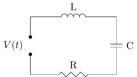
If we assume that the input voltage $V(t)$ is constant then $dV/dt=0$ and the current $I(t)$ satisfies \[L\dfrac{d^2I}{dt^2}+R\dfrac{dI}{dt}+\dfrac{I}{C}=0.\]

Equations of this type appear in many different situations. For instance, an equivalent mathematical model appears in the motion of a shock absorber, as follows. Suppose we have a mass $m$ attached to a spring and connected to a piston which resists the motion of the mass.

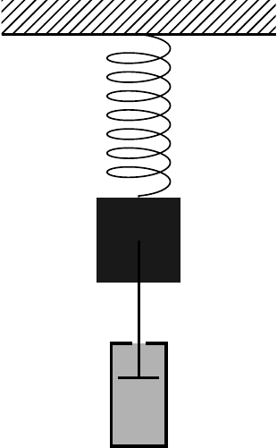
Then the position $y(t)$ of the mass at time $t$ satisfies \[m\dfrac{d^2y}{dt^2}+c\dfrac{dy}{dt}+ky=0\] where $k$ is the modulus of the spring and $c$ is the damping constant of the piston.

We will now use the results of the last sections to describe qualitatively the types of behaviour that such models can exhibit. In particular, for the damped spring system we introduce the following positive real parameters: \[\omega_0=\sqrt{\frac{k}{m}}\qquad\text{and}\qquad\zeta=\frac{c}{2\sqrt{mk}}.\]

Here $\omega_0$ is called the natural frequency and $\zeta$ is the damping ratio. The differential equation can then be written as \[\frac{d^2y}{dt^2}+2\zeta\omega_0\frac{dy}{dt}+\omega_0^2y=0.\]

Applying the method from the last section, the auxiliary equation is \[\lambda^2+2\zeta\omega_0\lambda+\omega_0^2=0\] which has solutions \[\lambda_1,\lambda_2=\frac{-2\zeta\omega_0\pm\sqrt{4\zeta^2\omega_0^2-4\omega_0^2}}{2} =-\zeta\omega_0\pm\omega_0\sqrt{\zeta^2-1}.\]

The three different cases of solutions thus correspond to $\zeta>1$, $\zeta=1$ and $\zeta<1$ respectively.

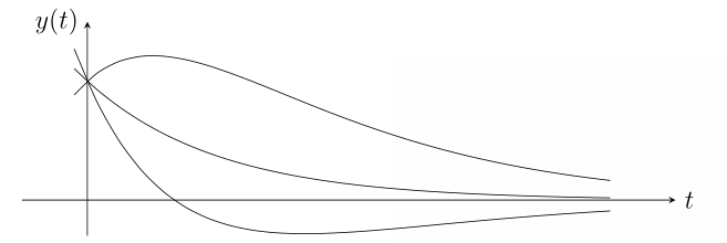
Overdamping ($\zeta>1$)$\;$ The roots $\lambda_1=-\zeta\omega_0+\omega_0\sqrt{\zeta^2-1}$ and $\lambda_2=-\zeta\omega_0-\omega_0\sqrt{\zeta^2-1}$ are distinct and real so the general solution is given by \[y(t)=Ae^{\lambda_1t}+Be^{\lambda_2t}.\] Notice that $\lambda_2<\lambda_1<0$ as the parameters $\omega_0$, $\zeta$ are positive and $\zeta=\sqrt{\zeta^2}>\sqrt{\zeta^2-1}$. Hence $y(t)$ is a sum of two decaying exponential terms and the motion rapidly decreases to zero. The following graph displays a few solutions with $y(0)$ fixed and various $y'(0)$.

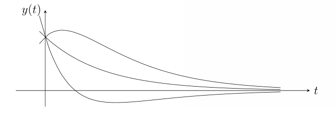
Critical damping ($\zeta=1$)$\;$ The two roots are equal to $\lambda=-\omega_0$ and the general solution is given by \[y(t)=(At+B)e^{\lambda t}.\] Since $\lambda<0$, the exponential term is decaying and the motion rapidly decreases to zero similarly to the previous case. The following graph displays a few possible solutions.

Underdamping ($0\leq\zeta<1$) $\;$ In this case, the two roots $\lambda_1=-\zeta\omega_0+\omega_0\sqrt{\zeta^2-1}$ and $\lambda_2=-\zeta\omega_0-\omega_0\sqrt{\zeta^2-1}$ are complex conjugates. In fact, if we write $\omega=\omega_0\sqrt{1-\zeta^2}$, then these two roots are \[\lambda_1,\lambda_2=-\zeta\omega_0\pm i\omega.\] Hence the general solution is given by \[y(t)=e^{-\zeta\omega_0 t}\left(A\cos{\omega t}+B\sin{\omega t}\right).\] This time, the solution consists of a decaying exponential term multiplied by a trigonometric term which oscillates with frequency $\omega$ (the actual frequency).

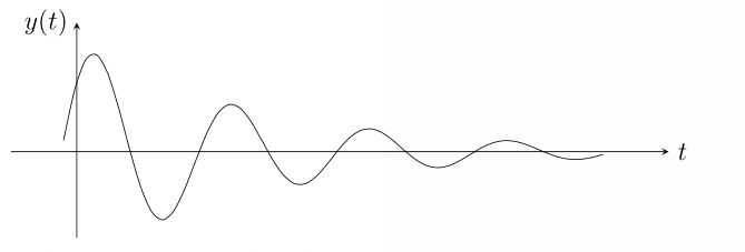
Remark. Note the special case of no damping $\zeta=0$ where we just get a sinusoidal wave with frequency $\omega_0$ and constant amplitude. This is simple harmonic motion.

Remark. One can also consider models that include a driving force. For instance, suppose the damped mass on a spring is also pushed by an external force $F(t)$ which varies over time. This leads to equations such as \[\frac{d^2y}{dt^2}+2\zeta\omega_0\frac{dy}{dt}+\omega_0^2y=\frac{F(t)}{m}.\] Here our method for solving the inhomogeneous case come into play and the behaviour will be dependent on the forcing function $F(t)$. We won’t go into detail about the more complicated solutions that now appear. But consider what happens in the underdamped case with a driving force $F(t)=mF_0\cos(\omega_d t)$ oscillating with some frequency $\omega_d$ and constant amplitude $mF_0$.

The general solution $y=y_c+y_p$ will consist of an exponentially decaying part $y_c$ with frequency $\omega$ together with a particular integral $y_p$. Over time, $y_c$ quickly tends to zero (it is transient), leaving just $y_p$ (the steady state).

Further interesting things can happen. Consider the special case with the same driving force but no damping, so that $y_c=A\cos{\omega t}+B\sin{\omega t}$. Then

If $\omega_d\neq \omega$ then $y_p=c\cos(\omega_dt)+d\sin(\omega_dt)$ is another sinusoidal wave with constant amplitude.
If $\omega_d=\omega$ then by the modification rule, $y_p=ct\cos(\omega_dt)+dt\sin(\omega_dt)$ which oscillates with growing amplitude. Careful analysis of this and similar types of behaviour leads to developing the concept of resonance. (Think about pushing somebody on a swing building up the amplitude with each push…)

6.9 Systems of Linear ODEs

In applications, differential equations often arise between several variables - these are generally very difficult to solve and often we can only give numerical solutions. For instance, the phugoid equations \[\frac{dv}{dt}=-\sin\theta-Rv^2,\qquad \frac{d\theta}{dt}=\frac{v^2-\cos\theta}{v}\] don’t have a closed-form general solution. However, when the equations are linear, we can use the matrix methods from last term to solve them exactly.

In what follows, we will have functions $x(t)$, $y(t)$,… of a variable $t$ and will write dots over them to signify their derivatives $\dot{x}=dx/dt$, $\dot{y}=dy/dt$,…

Example 6.21. Solve the following system of ODEs. \[\begin{align*} \dot{x}&=x-2y+2z \\ \dot{y}&=-x+y+z \\ \dot{z}&=-x-2y+4z \end{align*}\] Put ${\bf x}=\displaystyle\begin{pmatrix} x \\ y \\ z \end{pmatrix}$ and write the system in matrix form $\dot{{\bf x}}=A{\bf x}$. \[\dot{{\bf x}}=\begin{pmatrix} \dot{x} \\ \dot{y} \\ \dot{z} \end{pmatrix}= \begin{pmatrix} 1 & -2 & 2 \\ -1 & 1 & 1 \\ -1 & -2 & 4 \end{pmatrix} \begin{pmatrix} x \\ y \\ z \end{pmatrix} \] The trick is to then diagonalise the matrix $A$. We can write $Y^{-1}AY=D$ where \[Y=\begin{pmatrix} 1& 0 & 1 \\ 1 & 1 & 0 \\ 1 & 1 & 1 \end{pmatrix} \qquad\text{and}\qquad D=\begin{pmatrix} 1 & 0 & 0 \\ 0 & 2 & 0 \\ 0 & 0 & 3 \end{pmatrix}.\]

Exercise: Check this by finding the eigenvalues and eigenvectors of $A$ for yourself and putting the eigenvectors in the columns of $Y$.

Now create a new vector variable $\bf u=\displaystyle\begin{pmatrix} u \\ v \\ w \end{pmatrix}$ satisfying $Y{\bf u}={\bf x}$.

We then have $Y\dot{{\bf u}}=\dot{{\bf x}}$ and, moreover, \[Y\dot{{\bf u}}=\dot{{\bf x}}=A{\bf x}=AY{\bf u} \quad\implies\quad \dot{{\bf u}}=Y^{-1}AY{\bf u}=D{\bf u}.\] In terms of the coordinates, this says \[\begin{pmatrix} \dot{u} \\ \dot{v} \\ \dot{w} \end{pmatrix} =\begin{pmatrix} 1 & 0 & 0 \\ 0 & 2 & 0 \\ 0 & 0 & 3 \end{pmatrix} \begin{pmatrix} u \\ v \\ w \end{pmatrix} =\begin{pmatrix} u \\ 2v \\ 3w \end{pmatrix} \quad\implies\quad \begin{cases} \dot{u}=u \\ \dot{v}=2v \\ \dot{w}=3w \end{cases}\]

By diagonalising, we have decoupled the equations and they are now easy to solve: \[\begin{cases} \dot{u}=u \\ \dot{v}=2v \\ \dot{w}=3w \end{cases} \qquad\implies\qquad \begin{cases} u=ae^t \\ v=be^{2t} \\ w=ce^{3t} \end{cases}\] where $a,b,c$ are arbitrary constants. We can now find ${\bf x}=Y{\bf u}$: \[\begin{pmatrix} x \\ y \\ z \end{pmatrix}= \begin{pmatrix} 1 & 0 & 1 \\ 1 & 1 & 0 \\ 1 & 1 & 1 \end{pmatrix} \begin{pmatrix} ae^t\\ be^{2t} \\ ce^{3t} \end{pmatrix}= \begin{pmatrix} ae^t+ce^{3t} \\ ae^{t}+be^{2t} \\ ae^{t}+be^{2t}+ce^{3t} \end{pmatrix}\] Hence the general solution is $\;\;\;\begin{cases} \;x=ae^t+ce^{3t}, \\ \;y=ae^t+be^{2t}, \\ \;z=ae^t+be^{2t}+ce^{3t}. \end{cases}$

The method applies similarly if we are given differential equations with initial conditions. Find the general solution first and then apply the initial conditions to determine the unknown constants.

Example 6.22. Solve the system $\;\begin{cases} \;\dot{x}=11x-6y \\ \;\dot{y}=18x-10y\end{cases}\;\;$ where $x(0)=5$, $y(0)=9$.

First, rewrite the equations in matrix form: \[\dot{{\bf x}}=\begin{pmatrix} \dot{x} \\ \dot{y} \end{pmatrix} =\begin{pmatrix} 11 & -6 \\ 18 & -10 \end{pmatrix} \begin{pmatrix} x \\ y \end{pmatrix}=A{\bf x}.\] The characteristic polynomial of $A$ is \[\begin{align*} \begin{vmatrix} 11-\lambda & -6 \\ 18 & -10-\lambda \end{vmatrix} &=(11-\lambda)(-10-\lambda)+6\times 18 \\ &=\lambda^2-\lambda-2=(\lambda-2)(\lambda+1) \end{align*}\] so the eigenvalues are $\lambda=2$ and $-1$.

For $\lambda=-1$ we solve $(A+I){\bf v}={\bf 0}$, i.e.

\[\left(\begin{array}{cc|c} 12 & -6 & 0 \\ 18 & -9 & 0 \end{array}\right) \xrightarrow[(1/9)R_2]{(1/6)R_1} \left(\begin{array}{cc|c} 2 & -1 & 0 \\ 2 & -1 & 0 \end{array}\right) \xrightarrow{R_2-R_1} \left(\begin{array}{cc|c} 2 & -1 & 0 \\ 0 & 0 & 0 \end{array}\right).\] A corresponding eigenvector is ${\bf v}=\displaystyle\begin{pmatrix} 1 \\ 2 \end{pmatrix}$ (or any non-zero multiple of this).

For $\lambda=2$ we solve $(A-2I){\bf v}={\bf 0}$, i.e. \[\left(\begin{array}{cc|c} 9 & -6 & 0 \\ 18 & -12 & 0 \end{array}\right) \xrightarrow[(1/6)R_2]{(1/3)R_1} \left(\begin{array}{cc|c} 3 & -2 & 0 \\ 3 & -2 & 0 \end{array}\right) \xrightarrow{R_2-R_1} \left(\begin{array}{cc|c} 3 & -2 & 0 \\ 0 & 0 & 0 \end{array}\right).\] This time we may take corresponding eigenvector ${\bf v}=\displaystyle\begin{pmatrix} 2 \\ 3 \end{pmatrix}$.

Hence if we set $Y=\displaystyle\begin{pmatrix} 1 & 2 \\ 2 & 3 \end{pmatrix}$ and $D=\displaystyle\begin{pmatrix} -1 & 0 \\ 0 & 2 \end{pmatrix}$, then $Y^{-1}AY=D$.

Now make a new variable vector ${\bf u}=\displaystyle\begin{pmatrix} u \\ v \end{pmatrix}$ satisfying $Y{\bf u}={\bf x}$. Then \[Y\dot{{\bf u}}=\dot{{\bf x}}=A{\bf x}=AY{\bf u}\] and so \[\begin{pmatrix} \dot{u} \\ \dot{v} \end{pmatrix}= \dot{{\bf u}}=Y^{-1}AY{\bf u}=D{\bf u}= \begin{pmatrix} -1 & 0 \\ 0 & 2 \end{pmatrix} \begin{pmatrix} u \\ v \end{pmatrix} =\begin{pmatrix} -u \\ 2v \end{pmatrix}.\]

We now have two decoupled equations that we can solve separately: \[\begin{cases} \dot{u}=-u \\ \dot{v}=2v \end{cases} \quad\implies\quad \begin{cases} u=ae^{-t} \\ v=be^{2t} \end{cases}\] for some constants $a$ and $b$. The general solution is then found using ${\bf x}=Y{\bf u}$: \[\begin{align*} \begin{pmatrix} x \\ y \end{pmatrix} = \begin{pmatrix} 1 & 2 \\ 2 & 3 \end{pmatrix} \begin{pmatrix} ae^{-t} \\ be^{2t} \end{pmatrix}= \begin{pmatrix} ae^{-t}+2be^{2t} \\ 2ae^{-t}+3be^{2t} \end{pmatrix}. \end{align*}\] Now fitting the initial conditions gives the required solution: \[\begin{align*} \begin{cases} x(0)=a+2b=5 \\ y(0)=2a+3b=9 \end{cases} \;\;\implies\;\; \begin{cases} a=3 \\ b=1 \end{cases} \;\;\implies\;\; \begin{cases} x=3e^{-t}+2e^{2t}, \\ y=6e^{-t}+3e^{2t}. \end{cases} \end{align*}\]

For final practice, here’s a full (long) $3\times 3$ example.

Example 6.23. Solve the system $\;\begin{cases} \;\dot{x}=-2y+2z \\ \;\dot{y}=2y \\ \;\dot{z}=-x-y+3z \end{cases}$ given that $\;\begin{cases} \;x(0)=4, \\ \;y(0)=3, \\ \;z(0)=6. \end{cases}$

We first diagonalise the matrix of coefficients \[A=\begin{pmatrix} 0 & -2 & 2 \\ 0 & 2 & 0 \\ -1 & -1 & 3 \end{pmatrix}.\] Its eigenvalues are the solutions of \[\begin{align*} \det(A-\lambda I)&= \begin{vmatrix} -\lambda & -2 & 2 \\ 0 & 2-\lambda & 0 \\ -1 & -1 & 3-\lambda \end{vmatrix} =(2-\lambda)\begin{vmatrix}-\lambda & 2 \\ -1 & 3-\lambda \end{vmatrix} \\ &=(2-\lambda)(\lambda^2-3\lambda+2)=(1-\lambda)(2-\lambda)^2=0 \end{align*}\] and so the eigenvalues are $\lambda=1$, $2$, $2$.

For $\lambda=1$, we need to find ${\bf v}=\displaystyle\begin{pmatrix} v_1 \\ v_2 \\ v_3 \end{pmatrix}$ satisfying $(A-I){\bf v}={\bf 0}$: \[\begin{align*} \left(\begin{array}{ccc|c} -1 & -2 & 2 & 0 \\ 0 & 1 & 0 & 0 \\ -1 & -1 & 2 & 0 \end{array}\right) &\xrightarrow{R_3-R_1} \left(\begin{array}{ccc|c} -1 & -2 & 2 & 0 \\ 0 & 1 & 0 & 0 \\ 0 & 1 & 0 & 0 \end{array}\right) \\ &\xrightarrow[R_3-R_2]{R_1+2R_2} \left(\begin{array}{ccc|c} -1 & 0 & 2 & 0 \\ 0 & 1 & 0 & 0 \\ 0 & 0 & 0 & 0 \end{array}\right) \end{align*}\] which gives $-v_1+2v_3=0$ and $v_2=0$. Thus an eigenvector for $\lambda=1$ is $\displaystyle\begin{pmatrix} 2 \\ 0 \\ 1 \end{pmatrix}$.

For $\lambda=2$, we need to solve $(A-2I){\bf v}={\bf 0}$: \[\left(\begin{array}{ccc|c} -2 & -2 & 2 & 0 \\ 0 & 0 & 0 & 0 \\ -1 & -1 & 1 & 0 \end{array}\right) \xrightarrow{R_3-2R_1} \left(\begin{array}{ccc|c} -2 & -2 & 2 & 0 \\ 0 & 0 & 0 & 0 \\ 0 & 0 & 0 & 0 \end{array}\right)\] which means the eigenspace is given by just a single equation $v_1+v_2-v_3=0$. This is a plane and we would like to choose two independent eigenvectors on it. We can do this quickly by setting $v_1=1$, $v_2=0$ and $v_1=0$, $v_2=1$ to determine $v_3$.

We obtain two eigenvectors $\displaystyle\begin{pmatrix} 1 \\ 0 \\ 1 \end{pmatrix}$ and $\displaystyle\begin{pmatrix} 0 \\ 1 \\ 1 \end{pmatrix}$ which span the eigenspace for $\lambda=2$.

Putting this together, we find $Y^{-1}AY=D$ where \[Y=\begin{pmatrix} 2 & 1 & 0 \\ 0 & 0 & 1 \\ 1 & 1 & 1 \end{pmatrix} \qquad\text{and}\qquad D=\begin{pmatrix} 1 & 0 & 0 \\ 0 & 2 & 0 \\ 0 & 0 & 2 \end{pmatrix}. \]

Remember that this is not unique - for instance, changing the order of the eigenvalues and choosing different eigenvectors could lead you to \[Y=\begin{pmatrix} 1 & 2 & 4 \\ 0 & -1 & 0 \\ 1 & 1 & 2 \end{pmatrix} \qquad\text{and}\qquad D=\begin{pmatrix} 2 & 0 & 0 \\ 0 & 2 & 0 \\ 0 & 0 & 1 \end{pmatrix}\] which also satisfies $Y^{-1}AY=D$.

Now create a new vector variable $\bf u=\displaystyle\begin{pmatrix} u \\ v \\ w \end{pmatrix}$ satisfying $Y{\bf u}={\bf x}$. Then \[Y\dot{{\bf u}}=\dot{{\bf x}}=A{\bf x}=AY{\bf u} \quad\implies\quad \dot{{\bf u}}=Y^{-1}AY{\bf u}=D{\bf u}.\] This means that \[\begin{cases} \dot{u}=u \\ \dot{v}=2v \\ \dot{w}=2w \end{cases} \quad\implies\quad \begin{cases} u=ae^t \\ v=be^{2t} \\ w=ce^{2t} \end{cases}\] where $a,b,c$ are arbitrary constants. Thus $\;{\bf x}=Y{\bf u}=\displaystyle \begin{pmatrix} 2 & 1 & 0 \\ 0 & 0 & 1 \\ 1 & 1 & 1 \end{pmatrix} \begin{pmatrix} ae^t \\ be^{2t} \\ ce^{2t} \end{pmatrix}$

and the general solution is $\;\begin{cases} \;x=2ae^t+be^{2t}, \\ \;y=ce^{2t}, \\ \;z=ae^t+(b+c)e^{2t}. \end{cases}$

Finally, we use the initial conditions to determine $a$, $b$ and $c$. \[\begin{cases} x(0)=2a+b=4 \\ y(0)=c=3 \\ z(0)=a+b+c=6 \end{cases} \qquad\implies\qquad \begin{cases} a=1 \\ b=2 \\ c=2 \end{cases}\] and so the particular solution is $\;\begin{cases} \;x=2e^t+2e^{2t}, \\ \;y=3e^{2t}, \\ \;z=e^t+5e^{2t}. \end{cases}$

We can also occasionally use the method with higher order differential equations. For final final practice, let’s try an example.

Example 6.24. Find the general solution of the equations $\;\begin{cases} \;\ddot{x}=11x-6y, \\ \;\ddot{y}=18x-10y. \end{cases}$

Rewrite the equations in matrix form: \[\ddot{{\bf x}}=\begin{pmatrix} \ddot{x} \\ \ddot{y} \end{pmatrix} =\begin{pmatrix} 11 & -6 \\ 18 & -10 \end{pmatrix} \begin{pmatrix} x \\ y \end{pmatrix}=A{\bf x}\] Going through the usual diagonalisation process, one can find \[Y=\begin{pmatrix} 1 & 2 \\ 2 & 3 \end{pmatrix} \qquad\text{and}\qquad D=\begin{pmatrix} -1 & 0 \\ 0 & 2 \end{pmatrix}\] then $Y^{-1}AY=D$. Now set $Y{\bf u}={\bf x}$ so that \[Y\ddot{{\bf u}}=\ddot{{\bf x}}=A{\bf x}=AY{\bf u}\] Thus \[\begin{pmatrix} \ddot{u} \\ \ddot{v} \end{pmatrix}= \ddot{{\bf u}}=Y^{-1}AY{\bf u}=D{\bf u}= \begin{pmatrix} -1 & 0 \\ 0 & 2 \end{pmatrix} \begin{pmatrix} u \\ v \end{pmatrix} =\begin{pmatrix} -u \\ 2v \end{pmatrix}\]

We now have two decoupled 2nd order linear equations that we can solve separately using the methods of previous sections: \[\begin{cases} \ddot{u}+u=0 \\ \ddot{v}-2v=0 \end{cases} \quad\implies\quad \begin{cases} u=\alpha\cos{t}+\beta\sin{t} \\ v=\gamma e^{\sqrt{2}t}+\delta e^{-\sqrt{2}t} \end{cases}\] for some constants $\alpha$, $\beta$, $\gamma$ and $\delta$. Finally, we obtain the general solution using ${\bf x}=Y{\bf u}$: \[\begin{align*} x&=u+2v=\alpha\cos{t}+\beta\sin{t}+2\gamma e^{\sqrt{2}t}+2\delta e^{-\sqrt{2}t}, \\ y&=2u+3v=2\alpha\cos{t}+2\beta\sin{t}+3\gamma e^{\sqrt{2}t}+3\delta e^{-\sqrt{2}t}. \end{align*}\] If we had initial conditions, they would produce a linear system in $\alpha$, $\beta$, $\gamma$ and $\delta$ that we could solve with even more linear algebra!

\(r(x)\)	\(y_p(x)\)
\(ke^{\omega x}\)	\(Ce^{\omega x}\)
\(k_0+k_1x+\dots+k_nx^n\)	\(C_0+C_1x+\dots+C_nx^n\)
\(k\cos{\omega x}\)	\(C\cos{\omega x}+D\sin{\omega x}\)
\(k\sin{\omega x}\)	\(C\cos{\omega x}+D\sin{\omega x}\)