3 The multi-period binomial model

3.1 Model Description

We suppose all trading occurs at the times $t=0,1,\dots,T$, and that prices evolve between times $t$ and $t+1$ for $t=0,1,\dots,T-1$. As before, there is a risk-free asset with price $B_t$ that evolves deterministically, and there is a risky asset with price $S_t$ that evolves randomly.

The price dynamics of the risk-free asset represent the risk-free interest rate. The general model allows for the $B_t$’s to be any sequence of real numbers, but we will set \[ B_t = (1+r)^t, \quad t=0,\dots,T, \] so that $r$ is the (constant) interest rate over each time period $t$ to $t+1$.

We assume that $S_0$ is a fixed positive constant, and that for each $t$, given the current share price $S_t = s$, the new share price $S_{t+1}$ can take one of two values $su$ or $sd$ with probabilities $p_u$ and $p_d$. We note that the numbers $u$ and $d$ may in general depend on $t$ and $S_t$, but often we will assume that they are fixed constants. As with the one-period model we do not need to know the values of $p_u$ and $p_d$, only that $p_u,p_d > 0$ (and $p_u+p_d=1$). We can represent the dynamics of $S_t$ as a tree.

Example 3.1 Consider a two-period model with the possible share prices $S_t, t=0,1,2,$ given by the tree:

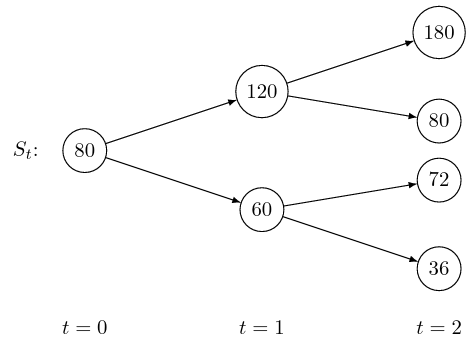
At $t=0$, we have $u=\frac{120}{80}=\frac{3}{2}$ and $d=\frac{60}{80}=\frac{3}{4}$.
At $t=1$, when $S_1=120$, we have $u=\frac{180}{120}=\frac{3}{2}$ and $d=\frac{80}{120}=\frac{2}{3}$.
At $t=1$, when $S_1 = 60$, we have $u=\frac{72}{60}=\frac{6}{5}$ and $d=\frac{36}{60}=\frac{3}{5}$.

A portfolio on a multi-period market is now more complicated to describe, since we need to specify the amounts we hold of each asset at each time $t$, and this is allowed to depend on how the share price changes over time. Despite this additional complication, we can price contingent claims on the multi-period model by applying the risk-neutral valuation formula at each node to get the no-arbitrage price, using a backwards induction (a bit like the idea of dynamic programming).

We focus on a single node of the tree at time $t$ and its two children at time $t+1$. Suppose the share price is at $S_t = s$ and goes to either $su$ or $sd$ at time $t+1$, and that we know the prices $\Pi^u_{t+1}$ and $\Pi^d_{t+1}$ of the contingent claim at the two nodes at time $t+1$.

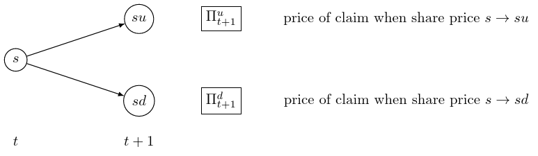
As in Chapter 2 the martingale probabilities at this node satisfy \[ s = \frac{1}{1+r} [q_u su + q_d sd ] \] and so $q_u = \displaystyle\frac{1+r-d}{u-d}, q_d = \frac{u-(1+r)}{u-d}$. Moreover, the price $\Pi_t$ at time $t$ is given by \[ \Pi_t = \frac{1}{1+r}[q_u \Pi^u_{t+1} + q_d \Pi^d_{t+1}]. \]

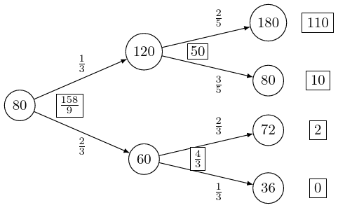
Example 3.2 For the market given in Example 3.1, with interest rate $r=0$, we calculate the fair price of a European call option with expiry date $T=2$ and strike price $K=70$. We find the martingale measures at each node, and then find the fair price of the option by working back to $t=0$ from the rightmost nodes.

At $t=0$, we have $q_u = {\displaystyle\frac{1-\frac34}{\frac32-\frac34}} = \frac13$ and $q_d = {\displaystyle\frac{\frac32-1}{\frac32-\frac34}} = \frac23$.
At $t=1$ when $S_1 = 120$, we have $q_u = {\displaystyle\frac{1-\frac23}{\frac32-\frac23}} = \frac25$ and $q_d = {\displaystyle\frac{\frac32-1}{\frac32-\frac23}} = \frac35$.
At $t=1$ when $S_1 = 60$, we have $q_u = {\displaystyle\frac{1-\frac35}{\frac65-\frac35}} = \frac23$ and $q_d = {\displaystyle\frac{\frac65-1}{\frac65-\frac35}} = \frac13$.
At $t=2$ the value of the call option is $(S_2-70)^+$, so is equal to $110,10,2$ or 0 when $S_2$ equals $180,80,72$ or 36, respectively.
At $t=1$, when $S_1=120$, we have $\Pi^u_2=110$, $\Pi^d_2=10$ so $\Pi_1 = \frac{1}{1+0}[ \frac25\times 110 + \frac35\times 10 ] = 50$.
At $t=1$, when $S_1=60$, we have $\Pi^u_2=2$, $\Pi^d_2=0$ so $\Pi_1 = \frac{1}{1+0}[ \frac23\times 2 + \frac13\times 0 ] = \frac43$.
At $t=0$, we have $\Pi^u_1=50$, $\Pi^d_1=\frac43$ so $\Pi_0 = \frac{1}{1+0}[ \frac13\times 50 + \frac23\times \frac43 ] = \frac{158}9$.

We calculate the no-arbitrage price of the call option to be $\frac{158}9$. We can record the calculations in a single tree. We write the share prices inside the nodes, the martingale probabilities along the arrows and the prices of the claim next to the nodes in rectangles.

3.2 Portfolios and the Self-Financing Condition

A portfolio or trading strategy in this financial market is a sequence $h_t=(x_t, y_t), t=1, \dots, T$ of pairs of random variables.

$x_t$ is the number of units of the risk-free asset in your portfolio at time $t-1$ and kept until time $t$.
$y_t$ is the number of units of risky asset in your portfolio at time $t-1$ and kept until time $t$.

The amounts $x_t$ and $y_t$ depend on the present and past history $S_0, S_1, \cdots, S_{t-1}$ of stock prices and therefore it is reasonable to assume that \[ x_t=f_x(S_0, S_1, \dots, S_{t-1}), \quad y_t = f_y(S_0,S_1,\dots,S_{t-1}) \] for some functions $f_x$ and $f_y$.

For a given portfolio $h$, we set $h_{T+1} = h_T$ (in other words, set $x_{T+1} = x_T$ and $y_{T+1} =y_T$), by convention.

We define the value of the portfolio $h$ at time $t=0,\dots,T$ by \[ V_t=x_{t+1}B_t+y_{t+1}S_t. \] In other words, for $t=0,\dots,T-1$, this is the value of the portfolio at time $t$ after the trade at time $t$ (and before the next price change). (The convention $x_{T+1} = x_T$ and $y_{T+1}=y_T$ means the formula is also valid for $t=T$.)

What happens between times $t-1$ and $t$? The value $V_{t-1} = x_tB_{t-1}+y_tS_{t-1}$ of the portfolio changes because the price of the bond changes from $B_{t-1}$ to $B_t$ and the price of the stock changes from $S_{t-1}$ to $S_t$ (so the portfolio is now worth $x_t B_t + y_tS_t$), and accordingly you want to adjust your holdings $(x_t,y_t)$ to new amounts $(x_{t+1}, y_{t+1})$ with the corresponding value \[ V_t=x_{t+1}B_t+y_{t+1}S_t. \] The adjustment will be self-financing if these two values are the same, in other words if \[\begin{equation} x_tB_t+y_tS_t=x_{t+1}B_t+y_{t+1}S_t. \tag{3.1} \end{equation}\] If (3.1) holds for all $t=1,\dots,T$, we say the portfolio is self-financing. This condition basically means that you cannot take out money from the portfolio or put in money to the portfolio: it should finance itself.

Remark. Using the expression for the value $V_t$ of the portfolio at time $t$, the self-financing constraint (3.1) can be rewritten as the condition \[\begin{equation} V_t-V_{t-1}=x_t(B_t-B_{t-1})+y_t(S_t-S_{t-1}). \tag{3.2} \end{equation}\] The financial meaning is that the change in the value $V_t-V_{t-1}$ of a self-financing trading strategy is due only to the gains/losses \[ x_t(B_t-B_{t-1})+y_t(S_t-S_{t-1}) \] due to price changes of the assets. Summing both sides of (3.2) over $t$ we obtain \[ V_T-V_0=\sum_{t=1}^T (V_t-V_{t-1})=\sum_{t=1}^T x_t[B_t-B_{t-1}]+\sum_{t=1}^T y_t[S_t-S_{t-1}]. \] You will see this form when we start to define stochastic integration and self-financing conditions in continuous time.

3.3 Pricing Contingent Claims by Hedging

As with the one-period binomial model, we start by considering European options, where the contingent claim $X$ is of the form $\Phi(S_T)$. We suppose the contract is initiated at time $0\le t\le T$ and let $\Pi_t(\Phi)$ denote the fair price at that time.

Remark. Recall that the function $\Phi(\cdot)$ is called the contract function. Generally speaking a contingent claim can be any random variable $X$ representing the payoff of a contract. It doesn’t have to be of the special form $X=\Phi(S_T)$. It is called a European option because the payoff $\Phi(S_T)$ depends on the price of the stock at the final date $T$. If the payoff depends on the past history of the stock price then it is no longer a European option. We have all types of options like Asian options, barrier options, look back options, etc. All these options are called exotic options and the payoff of them depends on past price history. We will see how to price these (including American options) later in the course. For now we just study claims of the form $\Phi(S_T)$.

The following theorem tells us the fair price $\Pi_t(\Phi)$ for each $t=0,1,\dots,T$.

Theorem 3.1 If there exists a self-financing trading strategy $h_t=(x_t, y_t), t=1,2,\dots,T+1,$ with value process \[ V_t=x_{t+1}B_t+y_{t+1}S_t, \quad \text{for $t=0,1,\dots,T$}, \] such that $V_T = \Phi(S_T)$ with probability 1, then for all $t = 0,1,\dots,T$, the price $\Pi_t(\Phi)$ at time $t$ for the contingent claim $\Phi(S_T)$ satisfies \[ V_t=\Pi_t(\Phi) \] or else there will be an arbitrage.

Proof. To see this first suppose $V_t<\Pi_t(\Phi)$ for some $t$. Then at time $t$ we sell the contingent claim for $\Pi_t(\Phi)$, buy the portfolio for $V_t$ and deposit the remaining cash $\Pi_t(\Phi)-V_t$ into the bank (equivalently, use the cash to buy the risk-free asset). Now, since the portfolio is self-financing, we can rebalance the portfolio as the asset prices evolve at no additional cost, so that at time $T$ the portfolio is worth $V_T$. Since $V_T = \Phi(S_T)$, our liability $\Phi(S_T)$ at time $T$ due to selling the contingent claim at time $t$ is exactly covered by the portfolio. But our money in the bank is now worth $[\Pi_t(\Phi)-V_t](1+r)^{T-t} > 0$ which is a risk-free profit.

Similarly, if $V_t > \Pi_t(\Phi)$, we can buy the contingent claim and sell the portfolio and obtain the risk-free money $[V_t-\Pi_t(\Phi)](1+r)^{T-t}>0$.

We can now construct the hedging portfolio and no-arbitrage price by backwards induction from $t=T$.

We know that $V_T = \Phi(S_T) = \Pi_T(\Phi)$, so we know the price of the claim at all nodes at time $T$.
Our inductive step is as follows. Suppose we have calculated the price $V_t=\Pi_t(\Phi)$ of the claim at all nodes at time $t$. We focus on a node at time $t-1$, and its two children at time $t$.

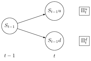
To satisfy the self-financing condition we need to find $x_t$ and $y_t$ with $x_tB_t+y_tS_t = V_t$ and this must hold whichever node we reach at time $t$. These two possibilities give us two equations in two unknowns: \[\begin{align*} x_t(1+r)B_{t-1} + y_t S_{t-1}u &= \Pi^u_t,\\ x_t(1+r)B_{t-1} + y_t S_{t-1}d &= \Pi^d_t, \end{align*}\] which we can solve to get \[\begin{equation} x_t = \frac{1}{(1+r)B_{t-1}}\frac{u\Pi^d_t - d\Pi^u_t}{u-d}, \quad y_t = \frac{\Pi^u_t-\Pi^d_t}{S_{t-1}u-S_{t-1}d}, \tag{3.3} \end{equation}\] and \[ \begin{split} \Pi_{t-1} = V_{t-1} = x_tB_{t-1} + y_tS_{t-1} &= \frac{1}{1+r}\frac{u\Pi^d_t - d\Pi^u_t}{u-d} + \frac{\Pi^u_t-\Pi^d_t}{u-d}\\ &= \frac{1}{1+r} [ q_u \Pi^u_t + q_d \Pi^d_t], \end{split} \] recalling that the martingale probabilities are $q_u = \displaystyle\frac{1+r-d}{u-d}, q_d = \frac{u-(1+r)}{u-d}$.

We can repeat these calculations at every node at time $t-1$ (noting that the values of $u$ and $d$ might be different at different nodes), to find the price $V_{t-1} = \Pi_{t-1}(\Phi)$ and the portfolio $(x_t,y_t)$ at every node at time $t-1$.

So, starting at time $T$, we use equations (3.3) to find $(x_T,y_T)$ at every node at time $T-1$ so that the value of the portfolio matches the prices $\Pi_T(\Phi)$ at time $T$. We calculate $V_{T-1}$ which then must be equal to the price of the claim $\Pi_{T-1}(\Phi)$ at time $T-1$. Then, using our inductive step for $t=T-1,T-2,\dots,1$, we can find the price of the claim and the portfolio at every node of the tree.

Remark. Although we worked out the values of $x_t$ and $y_t$ in order to find $V_{t-1}$ (and so also $\Pi_{t-1}$), we see that the expression we get for $\Pi_{t-1}$ only involves the values of $\Pi_t$ at the nodes at time $t$ and the relevant martingale probabilities. In other words, we can calculate all the martingale probabilities and fair prices at each node without needing to find the hedging portfolio — just as in the one-period case.

We now calculate the hedging or replicating portfolio for the call option from Example 3.2.

Example 3.3 We have already calculated in Example 3.2 the fair prices of the call option at each node and we can use these and the equations in (3.3) to find $(x_t,y_t)$ at each node.

At $t=0$, we need to find $(x_1,y_1)$ so that the value of the portfolio matches the two possible prices (50 or $4/3$) for the claim at time 1. Since $r=0$, we have $B_t = 1$ for all $t$, and so \[ x_1 = \frac{\frac32\times\frac43 - \frac34\times 50}{\frac32-\frac34} = -\frac{142}3,\quad y_1 = \frac{50 - \frac43}{120-60} = \frac{73}{90}, \] and $V_0 = x_1 + 80y_1 = -\frac{142}3 + 80\times\frac{73}{90} = \frac{158}9$.

Now, suppose that at time $t=1$, the stock price increases to 120. The portfolio $(x_1,y_1)$ is now worth $x_1 + 120y_1 = -\frac{142}3 + 120\times\frac{73}{90} = 50$ (which matches the price of the claim). We need to find the new amounts $(x_2,y_2)$ so that whatever happens the to the stock price at time 2 the portfolio matches the possible prices (110 or 10) of the claim at time 2. Again, using (3.3) and the appropriate values for $u$ and $d$ (remember these can be different at different nodes!) we get \[ x_2 = \frac{\frac32\times10 - \frac23\times 110}{\frac32-\frac23} = -70,\quad y_2 = \frac{110 - 10}{180-80} = 1, \] and $V_1 = x_2 + 120y_2 = -70 + 120\times 1 = 50$. We see that the value of this new portfolio $(x_2,y_2)$ is the same as that of $(x_1,y_1)$ as is required by the self-financing condition.

Now, we consider what can happen at time $t=2$. If the stock price increases to 180, then the portfolio becomes worth $x_2+180y_2 = -70 +180\times 1 = 110$, which matches the price of the call option. However, if the stock price decreases to 80, then the portfolio becomes worth $x_2+80y_2 = -70 + 80\times 1 = 10$, and again we have matched the price of the call option.

So, we have successfully matched the return given at time $t=2$ by the call option with a portfolio of bonds and stocks, in two of the possible four possibilities, when $S_2$ is either 180 or 80—in other words when, at time $t=1$, the stock price increases to 120. But what if the stock price decreases to 60 at time 1? In this case, we need different values for $(x_2,y_2)$ to match return of the call option (but this is allowed because $x_2$ and $y_2$ can depend on $S_0$ and $S_1$). Let’s do the calculations.

If the stock price decreases to 60 at time 1, the portfolio $(x_1,y_1)$ will then be worth $x_1 + 60y_1 = -\frac{142}3 + 60\times\frac{73}{90} = \frac43$ (matching the price of the claim at time 1). We now find $(x_2,y_2)$ so that the portfolio matches the possible prices (2 or 0) of the claim at time 2. Equations (3.3) give \[ x_2 = \frac{\frac65\times0 - \frac35\times 2}{\frac65-\frac35} = -2,\quad y_2 = \frac{2 - 0}{72-36} = \frac{1}{18}, \] and $V_1 = x_2 + 60y_2 = -2 + 60\times\frac1{18} = \frac43$, so again we satisfy the self-financing condition. Finally, we consider what can happen in this case at time $t=2$. We see that if the stock price increases from 60 to 72, then the portfolio becomes worth $x_2+72y_2 = -2 + 72\times\frac1{18} = 2$, which matches the price of the call option. Alternatively, if the stock price decreases from 60 to 36, then the portfolio becomes worth $x_2+36y_2 = -2 + 36\times\frac1{18} = 0$, again matching the price of the call option.

We have replicated the returns of the random variable $(S_T-70)^+$ using this self-financing portfolio.

We finish this section by noting that we can view the initial price $\Pi_0(\Phi)$ as the present value of the expectation of the random variable $\Phi(S_T)$, using the martingale measure for $S_T$, which can be obtained by multiplying the martingale probabilities along the edges from the start node at time 0 to the final nodes at time $T$. Equivalently, we know that the martingale measure $\Q$ for $S_T$ satisfies \[\begin{equation*} S_0 = \frac{1}{(1+r)^T} \E_\Q[S_T], \end{equation*}\] and with this measure we can write the price $\Pi_0(\Phi)$ as \[\begin{equation*} \Pi_0(\Phi) = \frac{1}{(1+r)^T} \E_\Q[\Phi(S_T)]. \end{equation*}\]

Example 3.4 Consider the market as described in Examples 3.1 and 3.2. Using the martingale probabilities on each arrow, we can calculate the martingale measure $\Q$ for $S_2$ (here $T=2$). For example, the stock price $S_2$ equals 180 exactly when the price $S_t$ follows the path $80 \to 120 \to 180$ through the tree, so $\Q[S_2 = 180] = \frac13\times\frac25 = \frac2{15}$. There are a total of 4 possible values that $S_2$ can take: 180, 80, 72 or 36, and these have probabilities $\frac2{15}, \frac15, \frac49$ and $\frac29$.

The expectation of $S_2$ with respect to this measure is $\E_\Q[S_2] = \frac2{15}\times 180 + \frac15 \times 80 +\frac49 \times 72 +\frac29 \times 36 = 80$. As expected this equals $S_0$, since in this example $r=0$.

Now, to find the price $\Pi_0$ at time 0 of the call option with strike price 70 and expiry date $T=2$, we calculate the present value of the expectation under $\Q$ of the value at time $T$ of the call option, $(S_2-70)^+$. We find that $\E_\Q[(S_2-70)^+] = \frac2{15}\times 110 + \frac15 \times 10 +\frac49 \times 2 +\frac29 \times 0 = \frac{158}9$, which agrees with our previous calculation.

3.4 Recombinant trees

In this section we consider the case where the numbers $u$ and $d$ do not depend on the time $t$ or the price $S_t$. This means, for example, that an “up”-move in the stock price, followed by a “down”-move has the same result as a “down”-move followed by an “up”-move. In this situation, we say that the tree is recombinant. (In reality, the diagram is no longer a tree.) Because of this recombining, in this model we have only $t+1$ nodes at time $t$ (compared with the $2^t$ nodes in the previous section). As before, we assume that $S_0$ is some fixed constant $s>0$, so we can represent the price dynamics with the diagram:

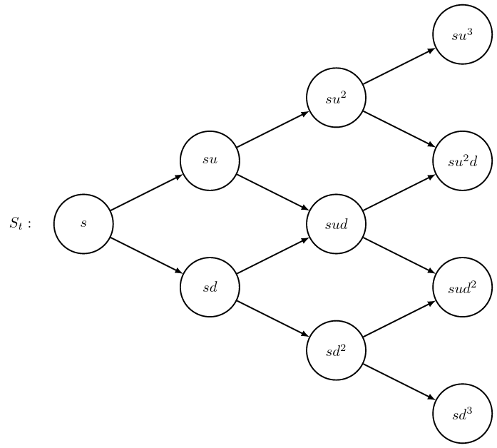
We see that the share price at time $t$ can be written as \[ S_t = s u^k d^{t-k}, \quad k=0,1,\dots,t, \] where $k$ denotes the total number of up-moves that have occurred (up to time $t$). This means that we can specify each node in the tree by a pair $(t,k)$ with $k=0,1,\dots,t$.

The contingent claim $\Phi(S_T)$ can be replicated using a self-financing portfolio. If $V_t(k)$ denotes the value of the portfolio at node $(t,k)$, then $V_t(k)$ can be computed recursively by \[\begin{equation} \begin{split} V_T(k) &= \Phi(su^kd^{T-k}), \\ V_t(k) &= \frac{1}{1+r}[q_u V_{t+1}(k+1) + q_d V_{t+1}(k)]. \end{split} \tag{3.4} \end{equation}\] where just as before $q_u$ and $q_d$ are the martingale probabilities at a node, given by \[ q_u = \frac{1+r-d}{u-d}, \quad q_d = \frac{u-(1+r)}{u-d}. \] We can also calculate the hedging portfolio, and writing $x_t(k)$ and $y_t(k)$ for the amounts held at node $(t-1,k)$, we have \[ x_t(k) = \frac{1}{(1+r)^t}\frac{uV_t(k) - dV_t(k+1)}{u-d}, \quad y_t(k) = \frac{V_t(k+1) - V_t(k)}{su^kd^{t-1-k}(u-d)}. \]

The recursive equations (3.4) are sometimes referred to as the binomial algorithm. We can use this algorithm to work out the fair price of a contingent claim at time 0, by starting with the nodes at time $t=T$ and working backwards to $t=0$. This gives us the following result.

Theorem 3.2 The arbitrage-free price at $t=0$ of a contingent claim $\Phi(S_T)$ is given by \[ \Pi_0(\Phi) = \frac{1}{(1+r)^T}\E_\Q(\Phi(S_T)), \] where $\Q$ is the martingale measure for $S_T$. More explicitly, we can write \[ \Pi_0(\Phi) = \frac{1}{(1+r)^T}\sum_{k=0}^T\binom{T}{k}q_u^kq_d^{T-k}\Phi(su^kd^{T-k}). \]

Proof. It is not difficult to see that the two expressions for $\Pi_0(\Phi)$ are equivalent. We know the martingale probabilities at each node are $q_u$ for an “up”-step, and $q_d$ for a “down”-step. Therefore, the martingale measure for $S_T$ can be calculated by determining the probability of reaching each node $(T,k)$, for $k = 0, \dots, T$. This is the probability that $S_T = S_0u^kd^{T-k}$, which happens if there are exactly $k$ “up”-steps out of the $T$ steps in total, and so has probability $\binom{T}{k} q_u^k q_d^{T-k}$. In other words, under the measure $\Q$, the price $S_T$ equals $S_0u^Yd^{T-Y}$, where $Y \sim \Bin(T,q_u)$, and therefore \[ \E_\Q[\Phi(S_T)] = \E[\Phi(S_0 u^Y d^{T-Y}) ] = \sum_{k=0}^T\Phi(S_0 u^kd^{T-k})\P[Y = k]. \] It is also easy to see that the explicit expression for $\Pi_0(\Phi)$ follows by applying the equations (3.4). Indeed, it is possible to show by induction on $t$, that the value $V_{T-t}(i)$ of the portfolio at a node $(T-t,i)$, for $T-t \in [0,T]$ and $i=0,\dots,T-t$, satisfies \[ V_{T-t}(i) = \frac{1}{(1+r)^t}\sum_{k=0}^t\binom{t}{k}q_u^kq_d^{t-k}\Phi(su^{i+k}d^{T-i-k}), \] and then by the Law of One Price, we have that $\Pi_0(\Phi) = V_0(0)$, which gives the required expression.

Exercise: work out the above proof by induction. Hint: in the inductive step use the identity $\binom{t}{k-1}+\binom{t}{k}=\binom{t+1}{k}$.

3.5 The Cox–Ross–Rubinstein formula

We use the pricing formula we found in the previous section to give a formula for the price of a European call option, known as the Cox–Ross–Rubinstein formula.

As usual, let $K$ be the strike price of the call option, and $T$ the expiry date. The Cox–Ross–Rubinstein formula for the price of such a call option, assumes that the underlying stock can be modelled by the recombinant tree model we studied in the previous section, for appropriate choices of $u, d$ and $r$. As it stands, we haven’t yet considered how suitable the binomial model is as a model of stock price fluctuations. We’ll look at this question in Chapter 5, but for now we suppose that we have some appropriately chosen values for $u, d$ and $r$, and we price the option in terms of these parameters.

We can use the formula from Theorem 3.2, to price the call option by setting $\Phi(S_T) = (S_T - K)^+$. In fact, we give a more general form, for the price at time $T-t \in [0,T]$.

Theorem 3.3 (Cox-Ross-Rubinstein formula) The price at time $T-t$ of a European call option with strike price $K$ and expiry date $T$, is given by \[\begin{equation} \Pi_{T-t} = S_{T-t} \sum_{k=k^\star}^t \binom{t}{k} m_u^k m_d^{t-k} - \frac{K}{(1+r)^t} \sum_{k=k^\star}^t \binom{t}{k} q_u^k q_d^{t-k}, \tag{3.5} \end{equation}\] where $q_u,q_d$ are the risk-neutral probabilities, $\displaystyle m_u = \frac{q_u u}{1+r}, m_d = \frac{q_d d}{1+r}$ and $k^\star$ is the smallest integer $k$ that satisfies \[\begin{equation} k \log\left(\frac{u}{d}\right) > \log\left(\frac{K}{S_{T-t}d^t}\right). \tag{3.6} \end{equation}\]

Proof. The price $\Pi_{T-t}(\Phi)$ at time $T-t$ of the claim $\Phi(S_T)$ is a function of the share price $S_{T-t}$ given by \[ \frac{1}{(1+r)^t} \sum_{k=0}^t \binom{t}{k} q_u^k q_d^{t-k} \Phi(S_{T-t}u^kd^{t-k}). \] Since $\Phi(x) = (x - K)^+$, the terms appearing in this sum will be zero unless $S_{T-t}u^kd^{t-k} > K$. We can rewrite this condition as $(u/d)^k > K/(S_{T-t}d^t)$, and since $u/d > 1$, there is a smallest integer $k^\star$ given by (3.6), such that if $k \geq k^\star$ then the condition is satisfied. (Note that if $k^\star > t$ then the sum becomes zero, and $\Pi_{T-t} = 0$.)

In other words, we can write the price of a European call option as \[ \Pi_{T-t} = \frac{1}{(1+r)^t}\sum_{k=k^\star}^t \binom{t}{k}q_u^kq_d^{t-k}(S_{T-t}u^kd^{t-k} - K) \] and multiplying out the bracket and using the expressions for $m_u$ and $m_d$ yields the formula (3.5).

Example 3.5 Consider a 3-period model with $u=1.2$, $d=0.8$ and $r=0.1$. Suppose the share price at time 0 is $S_0 = 100$. We calculate the CRR price at time 0 of a European call option with strike price 70 and expiry date $T=3$.

First, we calculate the martingale probabilities: \[ q_u = \frac{1.1 - 0.8}{1.2-0.8} = \frac34, \quad q_d = \frac{1.2 - 1.1}{1.2-0.8} = \frac14. \]

Then, we calculate $m_u$ and $m_d$: \[ m_u = \frac34\times\frac{1.2}{1.1} = \frac9{11}, \quad m_d = \frac14\times\frac{0.8}{1.1} = \frac2{11}. \]

To find the correct value of $k^\star$, we look at the possible values for the share price at time $T$. We see that $S_3$ can be one of 51.2, 76.8, 115.2 or 172.8, and so the call option only has positive value at time $T$ if at least one up-move occurs, so $k^\star = 1$.

(Alternatively, we can calculate $\log(K/S_0d^3) / \log(u/d) = \log(70/51.2) / \log(3/2) \approx 0.771$, and find that the smallest integer greater than this is $k^\star = 1$.)

Then the CRR price is given by \[ S_0 \sum_{k=1}^3 {\textstyle\binom{3}{k}} m_u^k m_d^{3-k} - \frac{K}{(1+r)^3} \sum_{k=1}^3 {\textstyle\binom{3}{k}} q_u^k q_d^{3-k} = 100\times \frac{1323}{1331} - \frac{70}{1.331} \times \frac{63}{64} = \frac{253575}{5324} \approx 47.63 \]

Remark. Note that $m_u, m_d > 0$ and $m_u+m_d = \displaystyle\frac{q_uu}{1+r} + \frac{q_dd}{1+r} = 1$, so that $m_u$ and $m_d$ can also be interpreted as probabilities. Hence we can write (3.5) as \[ \Pi_{T-t} = S_{T-t} \P[ X_t \geq k^\star ] - \frac{K}{(1+r)^t} \P[ Y_t \geq k^\star ], \] where $X_t$ and $Y_t$ are Binomial random variables: $X_t \sim \Bin(t,m_u), Y_t \sim \Bin(t,q_u)$.