Example 1.1 A chord of the unit circle is chosen at random. What is the probability that its length is larger than \(\sqrt{3}\), the side of the equilateral triangle inscribed in a circle?

Bertrand argued that there are at least three different but natural ways of generating a random chord:

• via “random endpoints”: choose two random points on the circumference of the circle and draw the chord joining them;

• via “random radial point”: choose a radius of the circle, choose a point on the radius and construct the chord through this point and perpendicular to the radius;

• via “random midpoint": choose a point anywhere within the circle and construct a chord with the chosen point as its midpoint.

It is an instructive exercise to compute the corresponding probabilities. For more details, see the Wiki page. \(\vartriangleleft\)

Example 1.2 In a standard coin-flipping experiment let \(A_k=\bigl\{\text{ first `head' occurs on $k$th flip}\bigr\}\) and \(B_n=\bigl\{\text{ `head' observed in the first $n$ flips}\bigr\}\); then \[B_n=\bigcup_{k=1}^n A_k,\qquad\text{ while }\qquad B_\infty\equiv \bigl\{\text{ `head' observed}\bigr\}=\bigcup_{k=1}^\infty A_k.\] \(\vartriangleleft\)

Definition 1.3 Let \(\mathcal{F}\) be a collection of subsets of \(\Omega\). We shall call \(\mathcal{F}\) a \(\sigma\)-field or a \(\sigma\)-algebra if it has the following properties:

1. \(\varnothing\in\mathcal{F}\);

2. if \(A\in\mathcal{F}\), then \(A^\mathsf{c}\in\mathcal{F}\);

3. if \(A_1\), \(A_2, \ldots\in\mathcal{F}\), then \(\bigcup_{k=1}^\infty A_k\in\mathcal{F}\).

Remark 1.3.1 As you know from Probability I, given \(\Omega\), the trivial \(\sigma\)-field \(\{\varnothing,\Omega\}\) is the smallest \(\sigma\)-field over \(\Omega\). Also, the collection of all subsets of \(\Omega\) (also known as the power set \(2^\Omega\)) is the largest \(\sigma\)-field over \(\Omega\). For further examples see your first year notes and Exercises  1.23- 1.25. \(\vartriangleleft\)

Definition 1.4 Let \(\Omega\) be a sample space, and \(\mathcal{F}\) be a \(\sigma\)-field of events in \(\Omega\). A probability distribution \(\mathsf{P}\) on \((\Omega,\mathcal{F})\) is a collection of numbers \(\mathsf{P}(A)\), \(A\in\mathcal{F}\), possessing the following properties:

1. for every event \(A\in\mathcal{F}\), \(\mathsf{P}(A)\ge0\);

2. \(\mathsf{P}(\Omega)=1\);

3. for any pair of incompatible events \(A\) and \(B\) (i.e., \(A\cap B=\varnothing\)), \(\mathsf{P}(A\cup B)=\mathsf{P}(A)+\mathsf{P}(B)\);

4. for any countable collection \(A_1\), \(A_2\), …of incompatible events (i.e., with \(A_i\cap A_j=\varnothing\) for \(i\neq j\)), \[\tag{1.1}\label{eq:countable-additivity} \mathsf{P}\Bigl(\bigcup_{k=1}^\infty A_k\Bigr)=\sum_{k=1}^\infty \mathsf{P}\bigl(A_k\bigr).\]

Remark 1.4.1 For the left-hand side of (\ref{eq:countable-additivity}) and (\ref{eq:countable-sub-additivity}) to make sense, the countable union \(\cup_{k=1}^\infty A_k\) must be an event. This is guaranteed by the assumption that \(\mathcal{F}\) is a \(\sigma\)-field. \(\vartriangleleft\)

Definition 1.5 A probability space is a triple \((\Omega,\mathcal{F},\mathsf{P})\), where \(\Omega\) is a sample space, \(\mathcal{F}\) is a \(\sigma\)-field of events in \(\Omega\), and \(\mathsf{P}(\cdot)\) is a probability measure on \((\Omega,\mathcal{F})\).

Example 1.6 If \(\Omega\) is countable, as is the case for a repeated coin flipping, we can set \((\Omega, 2^{\Omega},\mathsf{P})\) to be the probability space. Notice that for \(A \subset \Omega\), \(A=\bigcup_{\omega \in A} \{\omega\}\) so that \[\mathsf{P}(A)=\sum_{\omega \in A} \mathsf{P} (\{\omega\}).\] Then \(\mathsf{P}(\cdot)\) is uniquely defined from the individual values \(\mathsf{P} (\{\omega\})\).

More generally, let \(\Omega\) be a countable set and let \(p:\Omega \to [0,1]\) be such that \(\sum_{\omega \in \Omega}p(\omega)=1\). Then there exists a unique probability measure \(\mathsf{P}\) on \((\Omega,2^{\Omega})\) such that \(\mathsf{P}(\{\omega \})=p(\omega)\).

The case when \(\Omega\) is finite is especially simple. See your first year notes for more details! \(\vartriangleleft\)

Example 1.7 Let \(\mathcal{X}\) be an arbitrary set. If \(\mathcal{F}_1\) and \(\mathcal{F}_2\) are two \(\sigma\)-fields of subsets of \(\mathcal{X}\), then \(\mathcal{G}=\mathcal{F}_1\cap\mathcal{F}_2\) is also a \(\sigma\)-field of subsets of \(\mathcal{X}\).

To verify this simple but very important property, we just check that all conditions in Definition 1.3 are satisfied: 1) as \(\varnothing\in\mathcal{F}_i\) for all \(i\), we have \(\varnothing\in\mathcal{G}\), by the definition of the intersection of \(\mathcal{F}_i\); 2) fix arbitrary \(A\in\mathcal{G}\); then \(A\in\mathcal{F}_i\) and therefore \(A^\mathsf{c}\in\mathcal{F}_i\) for all \(i\) (as each \(\mathcal{F}_i\) is a \(\sigma\)-field), and so \(A^\mathsf{c}\in\mathcal{G}\), as before; 3) fix an arbitrary sequence \(A_1\), \(A_2, \ldots\in\mathcal{G}\); then \(A_1\), \(A_2, \ldots\in\mathcal{F}_i\) and therefore \(\bigcup_{k=1}^\infty A_k\in\mathcal{F}_i\) for all \(i\) (as each \(\mathcal{F}_i\) is a \(\sigma\)-field), and so \(\bigcup_{k=1}^\infty A_k\in\mathcal{G}\). \(\vartriangleleft\)

Definition 1.8 Let \(\mathcal{X}\) be an arbitrary set and let \(\mathcal{D}\) be an arbitrary collection of subsets of \(\mathcal{X}\). Let \(\mathcal{F}_\alpha\), \(\alpha\in\mathcal{A}\), be the collection of all sigma-fields in \(\mathcal{X}\) which contain \(\mathcal{D}\), namely \(\mathcal{D}\subset\mathcal{F}_\alpha\) for all \(\alpha\in\mathcal{A}\). Then \(\mathcal{G}:=\mathcal{G}_\mathcal{D}=\cap_{\alpha\in\mathcal{A}}\mathcal{F}_\alpha\) is the smallest sigma-field of subsets of \(\mathcal{X}\) containing \(\mathcal{D}\), also known as the \(\sigma\)-field generated by \(\mathcal{D}\).

Definition 1.9 The canonical probability space is the triple \(\bigl([0,1],\mathcal{B}[0,1],\mathsf{P}\bigr)\), where \(\mathcal{B}[0,1]\) is the Borel \(\sigma\)-field in \([0,1]\) and \(\mathsf{P}(\cdot)\) is the Lebesgue measure in \([0,1]\).

Remark 1.9.1 One can similarly define the Borel \(\sigma\)-field for other subsets \(\mathcal{X}\) of \(\mathbb{R}\) (including the positive half-line \([0,\infty)\) or the whole of \(\mathbb{R}\)). The length measure then uniquely extends to the Lebesgue measure on \(\mathcal{X}\) (of course, in general one doesn’t expect the probabilistic normalisation \(\mathsf{P}(\mathcal{X})=1\)). Generalisations to higher dimensions are also available. \(\vartriangleleft\)

Remark 1.9.2 The Borel \(\sigma\)-field \(\mathcal{B}[0,1]\) is, arguably, the most natural sigma-field in \([0,1]\). It is generated by many collections of subsets of \([0,1]\). E.g., one can start from any of the collections \(\bigl\{(a,b)\bigr\}\), \(\bigl\{[a,b)\bigr\}\), \(\bigl\{[a,b]\bigr\}\), \(\bigl\{(0,b)\bigr\}\), \(\bigl\{(0,b]\bigr\}\), \(\bigl\{[0,b)\bigr\}\), \(\bigl\{[0,b]\bigr\}\), with \(a\), \(b\) being real, rational, or dyadic rational (i.e., ratios of the type \(\frac{m}{2^n}\) with integer \(m\), \(n\)) and get \(\mathcal{B}[0,1]\) as the corresponding generated sigma-field. Other options include (sufficiently large) collections of open sets or of closed sets in \([0,1]\) etc. While \(\mathbb{R}\) contains many subsets which are not Borel, it is not immediate to construct one. \(\vartriangleleft\)

Definition 1.10 A sequence \((A_n)_{n\ge1}\) of events is increasing if \(A_n\subseteq A_{n+1}\) for all \(n\ge1\). It is decreasing if \(A_n\supseteq A_{n+1}\) for all \(n\ge1\).

Example 1.11 If \((A_n)_{n\ge1}\) is a sequence of arbitrary events in some probability space \((\Omega,\mathcal{F},\mathsf{P})\), then the sequence \((B_n)_{n\ge1}\) with \(B_n=\cup_{k=1}^nA_k\) is increasing.

We first notice that for all sets \(C\) and \(D\) we have \(C\subset C\cup D\). Indeed, by definition, \(x\in C\cup D\) if and only if \(x\) belongs to \(C\) or \(x\) belongs to \(D\). In particular, every \(x\in C\) also belongs to \(C\cup D\), equivalently, \(C\subset C\cup D\). On the other hand, \[B_{n+1}=A_1\cup A_2\cup \ldots \cup A_n\cup A_{n+1}\equiv B_n\cup A_{n+1}\] so that \(B_n\subset B_{n+1}\) for all \(n\ge1\), as claimed.

A similar claim holds for finite intersections along the sequence \(A_n\), see . \(\vartriangleleft\)

Remark 1.12.1 If \((A_n)_{n\ge1}\) is not a monotone sequence of events, the claim of the lemma is not necessarily true ( find a counterexample!). \(\vartriangleleft\)

Example 1.13 A standard six-sided die is tossed repeatedly. Let \(N_1\) denote the total number of ’ones’ observed. Assuming that the individual outcomes are independent, show that \(\mathsf{P}(N_1=\infty)=1\).
Solution. We show that \(\mathsf{P}(N_1<\infty)=0\) by using a monotone approximation. First, notice that \(\{N_1<\infty\}=\cup_{n\ge1}B_n\) with \(B_n=\left\{\text{no `ones' after $n$th toss}\right\}\), so it is enough to show that \(\mathsf{P}(B_n)=0\) for all \(n\). However, \(B_n=\cap_{m>0}C_{n,m}\) with \(C_{n,m}=\left\{\text{no `one' on tosses $n+1$, \dots, $n+m$}\right\}\) being a decreasing sequence, \(C_{n,m}\supset C_{n,m+1}\) for all \(m\ge1\). By straightforward counting, \(\mathsf{P}(C_{n,m})=(5/6)^m\) for all \(m\), \(n\). Because \(\mathsf{P}(C_{n,m})\to0\) as \(m\to\infty\), Lemma 1.12 implies \(\mathsf{P}(B_n)=\lim_{m\to\infty}\mathsf{P}(C_{n,m})=0\), as claimed. \(\vartriangleleft\)

Example 1.14 Let \((A_n)_{n\ge1}\) be an arbitrary sequence of events. As shown in Example 1.11 and , the union of these events can be written as a monotone increasing limit of their finite unions \(B_n\), \[\bigcup_{n\ge1}A_n=\bigcup_{n\ge1}B_n,\qquad\text{ where }\qquad B_n:=\bigcup_{m=1}^nA_m.\] Similarly, by and , the intersection of these events can be written as a monotone decreasing limit of their finite intersections \(C_n\), \[\bigcap_{n\ge1}A_n=\bigcap_{n\ge1}C_n,\qquad\text{ where }\qquad C_n:=\bigcap_{m=1}^nA_m.\] In particular, \(\mathsf{P}(\cup_{n\ge1}A_n)\) and \(\mathsf{P}(\cap_{n\ge1}A_n)\) are well defined. \(\vartriangleleft\)

Definition 1.15 Let \((\Omega,\mathcal{F},\mathsf{P})\) be a probability space. Two events \(A\), \(B\in\mathcal{F}\) are independent, if their joint probability factorises, \[\tag{1.7}\label{eq:independent-events-def} \mathsf{P}(A\cap B)=\mathsf{P}(A)\mathsf{P}(B).\]

Example 1.16 Let \(A\), \(B\in\mathcal{F}\) be two events, where \(B\) has vanishing probability. Then \(A\) and \(B\) are independent: \[\tag{1.8}\label{eq:zero-probability-event-independence} \mathsf{P}(B)=0\qquad\Longrightarrow\qquad \mathsf{P}(A\cap B)=\mathsf{P}(A)\mathsf{P}(B).\] Similarly, if \(A\) is arbitrary but \(\mathsf{P}(B)=1\), then \(A\) and \(B\) are independent: \[\tag{1.9}\label{eq:full-probability-event-independence} \mathsf{P}(B)=1\qquad\Longrightarrow\qquad \mathsf{P}(A\cap B)=\mathsf{P}(A)\mathsf{P}(B).\]

Indeed, as \(A\cap B\subset B\), by the monotonicity property (\ref{eq:probability-monotone-inclusion}) we have \(\mathsf{P}(A\cap B)=0\) and so (\ref{eq:zero-probability-event-independence}) follows trivially. Similarly, as \(A\setminus (A\cap B)=A\setminus B\subset\Omega\setminus B=B^\mathsf{c}\) with \(\mathsf{P}(B^\mathsf{c})=0\), by (\ref{eq:two-events-combining-probability}) we deduce that \(0\le\mathsf{P}(A)-\mathsf{P}(A\cap B)\le\mathsf{P}(B^\mathsf{c})=0\), equivalently, \(\mathsf{P}(A\cap B)=\mathsf{P}(A)\); hence, (\ref{eq:full-probability-event-independence}) follows trivially. \(\vartriangleleft\)

Definition 1.17 Let \((\Omega,\mathcal{F},\mathsf{P})\) be a probability space. A finite or infinite collection of events \((A_\alpha)_{\alpha\in\mathcal{A}}\) is (mutually) independent, if the probability of any finite sub-collection factorises, namely, for all integer \(k\ge1\) and all \(\alpha_1\), …, \(\alpha_k\in\mathcal{A}\), \[\tag{1.10}\label{eq:independent-event-collections-def} \mathsf{P}\Bigl(\bigcap_{\ell=1}^k A_{\alpha_\ell}\Bigr)=\prod_{\ell=1}^k\mathsf{P}\bigl(A_{\alpha_\ell}\bigr).\]

Remark 1.18.1 The continuity properties of cumulative distribution functions rely upon the fact that monotone uncountable unions (intersections) of events can be written as countable unions (intersections) of suitable events, for which the continuity Lemma 1.12 can be applied. \(\vartriangleleft\)

Example 1.19 Given the canonical probability space \(\bigl([0,1],\mathcal{B}[0,1],\mathsf{P}\bigr)\) consider the random variable \(X\) defined via \(X(\omega)=\omega\). Then

\(\mathsf{P}(X\in[a,b])\equiv |[a,b]|=b-a\), for all \(0\le a\le b\le1\), that is, \(X\) is uniformly distributed, \(X\sim\mathcal{U}[0,1]\). \(\vartriangleleft\)

Example 1.20 Let \(X\) be a random variable on some probability space \((\Omega,\mathcal{F},\mathsf{P})\) and let \(f:\mathbb{R}\to\mathbb{R}\) be a function. Assume that \[\tag{1.12}\label{eq:measurable-functions} {}^\forall y\in\mathbb{R},\qquad f^{-1}\bigl((-\infty,y]\bigr)\in\mathcal{B}(\mathbb{R}),\] where \(\mathcal{B}(\mathbb{R})\) is the Borel sigma-field in \(\mathbb{R}\). Then the combined map \(Y(\omega):=f(X(\omega))\) is a random variable. \(\vartriangleleft\)

Remark 1.20.1 By using the standard properties of inverse functions, one can show that the relation (\ref{eq:measurable-functions}) extends to \[\tag{1.13}\label{eq:measurable-functions-general-def} {}^\forall B\in\mathcal{B}(\mathbb{R}),\qquad f^{-1}\bigl(B\bigr)\equiv\bigl\{x\in\mathbb{R}:f(x)\in B\bigr\}\in\mathcal{B}(\mathbb{R}),\] see . Functions satisfying (\ref{eq:measurable-functions-general-def}) are called measurable. \(\vartriangleleft\)

Definition 1.21 Two random variables \(X\) and \(Y\) on the same probability space \((\Omega,\mathcal{F},\mathsf{P})\) are independent, if \[\tag{1.14}\label{eq:two-rvs-independence-cdf} {}^\forall x,y\in\mathbb{R},\qquad \mathsf{P}(X\le x,Y\le y)=\mathsf{P}(X\le x)\mathsf{P}(Y\le y).\]

Remark 1.21.1 As in Remark 1.9.2, one can show that the Borel sigma field \(\mathcal{B}(\mathbb{R})\) can be generated by the collection \(\bigl\{(-\infty,a]:a\in\mathbb{R}\bigr\}\). Consequently, the condition (\ref{eq:two-rvs-independence-cdf}) is equivalent to \[\tag{1.15}\label{eq:two-rvs-independence-Borel} \mathsf{P}(X\in B_x,Y\in B_y)=\mathsf{P}(X\in B_x)\mathsf{P}(Y\in B_y)\] for all Borel sets \(B_x\), \(B_y\) in \(\mathcal{B}(\mathbb{R})\). \(\vartriangleleft\)

Definition 1.22 An arbitrary collection of random variables \((X_\alpha)_{\alpha\in\mathcal{A}}\) on some probability space \((\Omega,\mathcal{F},\mathsf{P})\) is (mutually) independent, if any finite sub-collection of these variables is independent, namely, for all integer \(k\ge1\), all \(\alpha_1\), …, \(\alpha_k\in\mathcal{A}\), and all real \(x_1\), …, \(x_k\), \[\tag{1.16}\label{eq:independent-variable-collections-def} \mathsf{P}\bigl(X_{\alpha_1}\le x_{\alpha_1},\dots,X_{\alpha_k}\le x_{\alpha_k}\bigr)=\prod_{\ell=1}^k\mathsf{P}\bigl(X_{\alpha_\ell}\le x_{\alpha_\ell}\bigr).\]

Example 1.23 If \(X_1\) and \(X_2\) are independent random variables, while functions \(f_1:\mathbb{R}\to\mathbb{R}\) and \(f_2:\mathbb{R}\to\mathbb{R}\) satisfy (\ref{eq:measurable-functions}) or (\ref{eq:measurable-functions-general-def}), then \(Y_i(\omega):=f_i(X_i(\omega))\) are independent random variables. This property easily extends to any finite or infinite setting. \(\vartriangleleft\)

Example 1.24 Let \(X_1\), \(X_2\) be independent variables and let the functions \(f_1\), \(f_2\) be as in Example 1.23. In view of the measure factorisation properties (\ref{eq:two-rvs-independence-cdf})-(\ref{eq:two-rvs-independence-Borel}), it is straightforward to deduce that \[\mathsf{E}(X_1X_2)=\mathsf{E}(X_1)\mathsf{E}(X_2),\qquad\text{ similarly, }\qquad \mathsf{E}\bigl(f_1(X_1)f_2(X_2)\bigr)=\mathsf{E}\bigl(f_1(X_1)\bigr)\mathsf{E}\bigl(f_2(X_2)\bigr).\] \(\vartriangleleft\)

Example 1.25 Fix arbitrary \(A\in\mathcal{B}[0,1]\) and consider the corresponding indicator random variable \(\mathbf{1}_A\). The latter is Bernoulli distributed with parameter \(\mathsf{E}\mathbf{1}_A=\mathsf{P}(\mathbf{1}_A=1)=\mathsf{P}(A)\), the Lebesgue measure of \(A\).

Fix arbitrary \(A\), \(B\in\mathcal{B}[0,1]\). Then \[\tag{1.17}\label{eq:set-operations-via-indicators} \mathbf{1}_{A\cap B}(\omega)\equiv \mathbf{1}_A(\omega)\mathbf{1}_B(\omega),\qquad \mathbf{1}_{A^\mathsf{c}}(\omega)\equiv 1-\mathbf{1}_A(\omega),\qquad \mathbf{1}_{A\cup B}(\omega)\equiv \mathbf{1}_A(\omega)+\mathbf{1}_B(\omega)-\mathbf{1}_{A\cap B}(\omega),\] and so all set operations can be recorded as linear combinations of products of indicator functions. Furthermore, it is straightforward to check that \[\tag{1.18}\label{eq:independence-of-events-and-their-indicators} \text{ events $A$ and $B$ are independent }\quad\Longleftrightarrow\quad\text{ random variables $\mathbf{1}_A$ and $\mathbf{1}_B$ are independent.}\] Indeed, by the above, for all \(C\), \(D\in\mathcal{B}[0,1]\) \[\tag{1.19}\label{eq:independence-of-events-via-their-indicators} \begin{gathered} \mathsf{P}(\mathbf{1}_C=1,\mathbf{1}_D=1)=\mathsf{P}(\mathbf{1}_C\mathbf{1}_D=1)=\mathsf{P}(\mathbf{1}_{C\cap D}=1)=\mathsf{P}(C\cap D), \quad\mathsf{P}(C)\mathsf{P}(D)=\mathsf{P}(\mathbf{1}_C=1)\mathsf{P}(\mathbf{1}_D=1) \end{gathered}\] with both expressions coinciding in the case where \(C\) and \(D\) are independent. Applying these relations to all combinations with \(C\in\{A,A^\mathsf{c}\}\) and \(D\in\{B,B^\mathsf{c}\}\) one deduces (\ref{eq:independence-of-events-and-their-indicators}). \(\vartriangleleft\)

Example 2.1 If events \((A_n)_{n\ge1}\) form an increasing sequence, then for each fixed \(\omega\in\Omega\) the real sequence \((x_n)_{n\ge1}\) with \(x_n:=\mathbf{1}_{A_n}(\omega)\in\{0,1\}\) is non-decreasing, and therefore converges.⁶

In particular, there are only three possibilities:
a) \(x_n=0\) for all \(n\ge1\), that is, \(\omega\) is outside of each set \(A_n\) and their limit \(A:=\lim_nA_n=\cup_nA_n\);
b) \(x_n=1\) for all \(n\ge1\), that is, \(\omega\) belongs to each \(A_n\) and to the limit set \(A\);
c) there is \(k\ge1\) such that \(x_1=\ldots=x_{k-1}=x_k=0\) while \(x_{k+1}=x_{k+2}=\ldots=1\), that is, \(\omega\) belongs to all but finitely many \(A_n\) and to the limit set \(A\).
E.g., in the setting of , if \(\Omega=[0,1]\) and \(A_n=[\tfrac1n,1]\) for \(n\ge1\), then \(A_n\) increases to \(A=(0,1]\) as \(n\to\infty\). Taking \(\omega\in\{0,\tfrac12,1\}\subset[0,1]\), we observe all three possibilities mentioned above. \(\vartriangleleft\)

Example 2.2 Let \(X\) be a positive random variable with \(\mathsf{P}(X<\infty)=1\). For \(n\ge1\), denote \(X_n=\frac1nX\) and, for \(\varepsilon>0\), let \(A_n(\varepsilon):=\bigl\{\omega:|X_n(\omega)|>\varepsilon\bigr\}\equiv\{|X|>n\varepsilon\}\). We obviously have \(A_n(\varepsilon)\supseteq A_{n+1}(\varepsilon)\) for fixed \(\varepsilon>0\) and all \(n\ge1\). Therefore, \[\bigcap_{n\ge1} A_n(\varepsilon)=\lim_{n\to\infty} A_n(\varepsilon)\equiv\bigl\{X=\infty\bigr\},\] which has probability zero by the assumption that \(\mathsf{P}(X<\infty)=1\). On the other hand, because \(A_n(\varepsilon)\) is a decreasing sequence, the event \[\bigl\{A_n(\varepsilon)\text{ i.o.}\bigr\}=\bigcap_{m\ge1}\bigcup_{n\ge m}A_n(\varepsilon) \equiv\bigcap_{m\ge1}A_m(\varepsilon)=\bigl\{X=\infty\bigr\}\] has probability zero. By taking complement, we conclude that \(\bigl\{A_n(\varepsilon)\text{ f.o.}\bigr\}\equiv\bigl\{X<\infty\bigr\}\) for each \(\varepsilon>0\). \(\vartriangleleft\)

Remark 2.2.1

Recall that the events \(A(\varepsilon)\equiv\bigl\{A_n(\varepsilon)\text{ f.o.}\bigr\}\equiv\bigl\{X<\infty\bigr\}\) in Example 2.2 do not depend on \(\varepsilon\). As a result, the convergence event,⁸

\[C:=\bigl\{\omega:X_n(\omega)\to0\bigr\}\equiv\bigcap_{\varepsilon>0}\bigl\{A_n(\varepsilon)\text{ f.o.}\bigr\}\equiv\bigl\{X<\infty\bigr\},\] has probability one. For this reason we say that the random variables \(X_k\) converge to zero with probability one (or almost surely). Different modes of convergence of random variables will be discussed later this term. \(\vartriangleleft\)

Remark The independence condition in part  b) above cannot be relaxed. Otherwise, let \(A_n\equiv E\) for all \(n\ge1\), where \(E\in\mathcal{F}\) satisfies \(0<\mathsf{P}(E)<1\) (and thus the events \(A_k\) are not independent). Then \(A=E\) and \(\mathsf{P}(A)=\mathsf{P}(E)\neq1\). \(\vartriangleleft\)

Remark An even more interesting counterexample to part b) without the independence property can be constructed as follows ( check this!):
\(\vartriangleleft\)

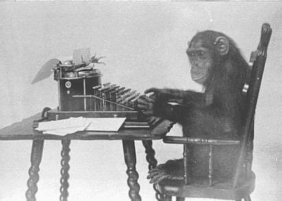
Example 2.4 By the second Borel-Cantelli lemma, Lemma 2.3 b), a monkey hitting keys at random on a typewriter keyboard for an infinite amount of time will almost surely (ie., with probability one) type any particular chosen text, such as the complete works of William Shakespeare (and, in fact, infinitely many copies of the chosen text).

Idea of the argument. Suppose that the typewriter has \(50\) keys, and the word to be typed is ‘banana’. The chance that the first letter typed is b is \(1/50\), as is the chance that the second letter is a, and so on. These events are independent, so the chance of the first six letters matching ‘banana’ is \(1/50^6\). For the same reason the chance that the next six letters match ‘banana’ is also \(1/50^6\), and so on.

Now, the chance of not typing ‘banana’ in each block of six letters is \(1-1/50^6\). Because each block is typed independently, the chance of not typing ‘banana’ in any of the first \(n\) blocks of six letters ¹⁰ is \(p=(1-1/50^6)^n\). If we were to count occurences of ‘banana’ that crossed blocks, \(p\) would approach zero even more quickly. ¹¹ Finally, once the first copy of the word ‘banana’ appears, the process starts afresh independently of the past, so that the probability of obtaining the second copy of the word ‘banana’ within the same number of blocks is still \(p\) etc.; the result now follows from Lemma 2.3.
Of course, the same argument applies if the monkey were typing any other string of characters of finite length, eg., your favourite novel. ¹² \(\vartriangleleft\)

Remark By using an appropriate monotone approximation, one can deduce the result as in Example 1.13, without explicitly using the Borel-Cantelli lemma. Moreover, the same argument can be extended to the situations, when the probability \(p_n\) of typing ‘banana’ in the \(n\)th block of six letters varies with \(n\), but remains uniformly positive, ie., \(p_n\ge\delta>0\) for all \(n\ge1\). The true power of the lemma is seen in the situations when \(p_n\to0\) slowly enough to have \(\sum_np_n=\infty\) (provided the events in different blocks are independent). \(\vartriangleleft\)

Example 2.5 A standard six-sided die is tossed repeatedly. Let \(N_k\) denote the total number of tosses when face \(k\) was observed. Assuming that the individual outcomes are independent, show that \[\mathsf{P}(N_1=\infty)=\mathsf{P}(N_2=\infty)=\mathsf{P}(N_1=\infty,N_2=\infty)=1.\]

Solution. Equalities \(\mathsf{P}(N_1=\infty)=\mathsf{P}(N_2=\infty)=1\) can be derived as in Example 1.13, so that the intersection event \(\{N_1=\infty,N_2=\infty\}\) has probability one.
Alternatively, we derive the first equality from the Borel-Cantelli lemma. To this end, fix \(k\in\{1,2,\dots,6\}\) and denote \(A_n^k=\left\{\text{$n$th toss shows $k$}\right\}\). For different \(n\), the events \(A_n^k\) are independent and have the same probability \(1/6\). As \(\sum_n\mathsf{P}(A_n^k)=\infty\), the Borel-Cantelli lemma implies that the event \(\bigl\{N_k=\infty\bigr\}\equiv\left\{A_n^k\text{ infinitely often}\right\}\) has probability one. The remaining claims now follow as indicated above. \(\vartriangleleft\)

Example 2.6 A coin showing ‘heads’ with probability \(p\) is tossed repeatedly. With \(X_n\) denoting the result of the \(n\)th toss, let \(C_n=\{X_n=T,X_{n-1}=\mathsf{H}\}\). Show that \(\mathsf{P}(C_n\text{ i.o.})=1\).
Solution. We have \({\{\text{$C_{2n}$ i.o.}\}}\subset\left\{\text{$C_{n}$ i.o.}\right\}\), where \(\mathsf{P}(C_{2n})\equiv pq\) and \(C_{2n}\) are independent. The result follows from Lemma 2.3 b) (or via monotone approximation). \(\vartriangleleft\)

Example 2.7 Let \((X_k)_{k\ge1}\) be  random variables with common exponential distribution of mean \(1/\lambda\),  \(\mathsf{P}\bigl(X_1>x\bigr)=e^{-\lambda x}\) for all \(x\ge0\). One can show that \(X_n\) grows like \(\frac1\lambda\log n\), more precisely, that ¹³ \[\mathsf{P}\bigl(\limsup_{n\to\infty}\tfrac {X_n}{\log n}=\tfrac1\lambda\bigr)=1.\]

Solution. For \(\varepsilon>0\), denote \[A_n^\varepsilon:=\Bigl\{\omega:X_n(\omega)>\tfrac{1+\varepsilon}\lambda\log n\Bigr\},\qquad B_n^\varepsilon:=\Bigl\{\omega:X_n(\omega)>\tfrac{1-\varepsilon}\lambda\log n\Bigr\}.\] We clearly have \(\mathsf{P}\bigl(A_n^\varepsilon\bigr)=n^{-(1+\varepsilon)}\) and \(\mathsf{P}\bigl(B_n^\varepsilon\bigr)=n^{-(1-\varepsilon)}\). As \(\sum_n\mathsf{P}(A_n^\varepsilon)<\infty\), by Lemma 2.3 a) the event \(\{\text{$A_n^\varepsilon$ infinitely often}\}\) has probability zero. Similarly, \(B_n^\varepsilon\) are independent and \(\sum_n\mathsf{P}(B_n^\varepsilon)=\infty\); thus, by Lemma 2.3 b), the event \(\{\text{$B_n^\varepsilon$ infinitely often}\}\) has probability one.

As for all \(n\ge1\) the events \(B_n^\varepsilon\) increase with \(\varepsilon\), the event \(B^*(\varepsilon):=\cap_{\varepsilon>0}\{\text{$B_n^\varepsilon$ infinitely often}\}\) has probability one. Similarly, for all \(n\ge1\) the events \(A_n^\varepsilon\) decrease with \(\varepsilon\), and therefore the event \(A^*(\varepsilon):=\cap_{\varepsilon>0}\{\text{$A_n^\varepsilon$ finitely often}\}\) also has probability one. By the characterization of \(\limsup\) (see, e.g., Lemma A.3), we finally deduce that \[\Bigl\{\limsup_{n\to\infty}\tfrac {X_n}{\log n}=\tfrac1\lambda\Bigr\} \equiv\bigcap_{\varepsilon>0}\bigl(\{\text{$A_n^\varepsilon$ finitely often}\}\cap\{\text{$B_n^\varepsilon$ infinitely often}\}\bigr) =\bigcap_{\varepsilon>0}\bigl(A^*(\varepsilon)\cap B^*(\varepsilon)\bigr),\] which is an event of probability one. \(\vartriangleleft\)

Remark 2.7.1 A slightly more general version of the argument in Example 2.7 allows to control the limiting behaviour of records:
Let \((X_k)_{k\ge1}\) be i.i.d. exponential r.v. with distribution \(\mathsf{P}(X_k>x)=e^{-x}\), and let \(M_n:=\max_{1\le k\le n}X_k\). Then \(\mathsf{P}(\tfrac{M_n}{\log n}\to1)=1\), ie., the normalized maximum \(\tfrac{M_n}{\log n}\) converges to \(1\) almost surely (as \(n\to\infty\)), see Figure  4. \(\vartriangleleft\)

Example 2.8 Let variables \((X_n)_{n\ge1}\) be i.i.d. with \(X_1\sim\mathcal{U}[0,1]\). For \(\alpha>0\), we have \(\mathsf{P}\bigl(X_n>1-n^{-\alpha}\bigr)=n^{-\alpha}\), so that \(\mathsf{P}\bigl(X_n>1-n^{-\alpha}\text{ i.o. }\bigr)=1\) iff \(\alpha\le1\).

A similar analysis shows that \[\mathsf{P}\Bigl(X_n>1-\frac1{n(\log n)^{\beta}}\text{ i.o.}\Bigr)=\begin{cases}1,&\quad \beta\le1,\\0,&\quad\beta>1.\end{cases}\] \(\vartriangleleft\)

Example 2.9 If \((X_k)_{k\ge1}\) is a sequence of random variables such that for every \(\varepsilon>0\) the event \[A(\varepsilon)\equiv\bigl\{|X_k|>\varepsilon\text{ finitely often}\bigr\}\] has probability one, then \(X_k\) is said to converge to zero with probability one, recall Remark 2.2.1.
As a simple illustration, let \(X_k=\frac1kX\), where a variable \(X\ge0\) has finite mean, \(\mathsf{E} X<\infty\). One then can show that, for each \(\varepsilon>0\), \[\sum_{k\ge1}\mathsf{P}(|X_k|>\varepsilon)=\sum_{k\ge1}\mathsf{P}(X>k\varepsilon)<\infty,\] and thus by Lemma 2.3 the event \(A(\varepsilon)\equiv\{|X_k|>\varepsilon\text{ f.o.}\}\) has probability one, for all such \(\varepsilon\). By the discussion in Remark 2.2.1 and monotonicity of \(A(\varepsilon)\), the convergence event, \(C=\cap_{\varepsilon>0} A(\varepsilon)\), has probability one.
A more general result in the setting of the amost sure convergence will be discussed later this term. \(\vartriangleleft\)

Definition 3.1 We say that a sequence of random variables \((X_n)_{n \geq 1}\) converges pointwise or surely to \(X\) if \(X_n(\omega) \to X(\omega)\) for all \(\omega \in \Omega\) as \(n \to \infty\).

Remark 3.1.1 The pointwise convergence is a very natural property. In particular, it is preserved ¹⁷ by the action of continuous functions: if \(X_n\to X\) surely as \(n\to\infty\), and \(f:\mathbb{R}\to\mathbb{R}\) is continuous, then the sequence \(\bigl(f(X_n)\bigr)_{n\geq1}\) of random variables converges to \(f(X)\) surely, cf. Lemma A.5.

However, pointwise convergence is a very restrictive condition and is often too strong to do anything useful in probability, even though this is the usual definition you might be familiar with from analysis courses. \(\vartriangleleft\)

Definition 3.2 For fixed \(r>0\), let \(X\) and \((X_n)_{n\ge1}\) be random variables such that \(\mathsf{E}(|X|^r)\) and all \(\mathsf{E}(|X_n|^r)\) are finite. Then the sequence \(X_n\) converges to \(X\) in \(L^r\) as \(n\to\infty\) (written \(X_n\stackrel{\mathsf{L}^r}{\to} X\)), if \(\mathsf{E}\bigl(|X_n-X|^r\bigr)\to0\) as \(n\to\infty\).

Remark 3.2.1 Such convergence is also known as convergence in the \(r\)-th mean. Two special cases are of particular importance.

When \(r=1\), the sequence \((X_n)_{n\ge1}\) converges to \(X\) in mean or in \(L^1\).

Similarly, when \(r=2\), the sequence \((X_n)_{n\ge1}\) converges to \(X\) in mean square or in \(L^2\). \(\vartriangleleft\)

Example 3.3 Let \(\bigl(X_n\bigr)_{n\ge1}\) be a sequence of random variables such that for some real numbers \((a_n)_{n\ge1}\), we have \[\tag{3.1}\label{eq:01-Lp-conv} \mathsf{P}\bigl(X_n=a_n\bigr)=p_n,\qquad \mathsf{P}\bigl(X_n=0\bigr)=1-p_n.\] Then \(X_n\stackrel{\mathsf{L}^r}{\to}0\) if and only if \(\mathsf{E}\bigl(|X_n|^r\bigr)\equiv|a_n|^rp_n\to0\) as \(n\to\infty\). \(\vartriangleleft\)

Definition 3.4 We say that a sequence \((X_n)_{n\ge1}\) of random variables converges to a random variable \(X\) in probability (write \(X_n\stackrel{\mathsf{P}}{\to} X\)) as \(n\to\infty\), if for every fixed \(\varepsilon>0\) \[\mathsf{P}\bigl(|X_n-X|\ge\varepsilon\bigr)\to0\qquad\text{ as }n\to\infty.\]

Remark 3.4.1 Convergence in probability is preserved under the action of continuous functions: If \(X_n\stackrel{\mathsf{P}}{\to} X\) as \(n\to\infty\) and \(f:\mathbb{R}\to\mathbb{R}\) is continuous, then \(f(X_n)\stackrel{\mathsf{P}}{\to} f(X)\) as \(n\to\infty\), cf. Lemma A.5. \(\vartriangleleft\)

Example 3.5 Let random variables \(\bigl(X_n\bigr)_{n\ge1}\) be as in (\ref{eq:01-Lp-conv}). Then for every \(\varepsilon>0\) we have \[\mathsf{P}\bigl(|X_n|\ge\varepsilon\bigr)\le\mathsf{P}\bigl(X_n\neq0)=p_n,\] so that \(X_n\stackrel{\mathsf{P}}{\to}0\) if \(p_n\to0\) as \(n\to\infty\). \(\vartriangleleft\)

Remark 3.6.1 Of course, (\ref{eq:general-Markov-inequality}) is trivial unless \(\mathsf{E}\bigl(g(X)\bigr)<\infty\).

When \(g(x)\equiv x\) for \(x\ge0\), (\ref{eq:general-Markov-inequality}) becomes Markov’s inequality. Similarly, when \(g(x)=x^2\) for \(x\ge0\) and \(X=|Y-\mathsf{E} Y|\) for some random variable \(Y\), (\ref{eq:general-Markov-inequality}) becomes Chebyshev’s inequality. \(\vartriangleleft\)

Example 3.8 Let random variables \((X_n)_{n\ge1}\) be as in (\ref{eq:01-Lp-conv}), where \(p_n\to0\) while \(|a_n|^rp_n\to\infty\) as \(n\to\infty\). Then, by Example 3.5, \(X_n\stackrel{\mathsf{P}}{\to}0\), while by Example 3.3, \(X_n\) does not converge to \(X\equiv0\) in \(L^r\). \(\vartriangleleft\)

Definition 3.9 A sequence \((X_k)_{k\ge1}\) of random variables in \((\Omega,\mathcal{F},\mathsf{P})\) converges, as \(n\to\infty\), to a random variable \(X\) with probability one (or almost surely) if \[\tag{3.3}\label{eq:convergence-almost-sure} \mathsf{P}\Bigl(\bigl\{\omega\in\Omega:X_n(\omega)\to X(\omega)\text{ as $n\to\infty$}\bigr\}\Bigr)=1.\]

Remark 3.9.1 For \(\varepsilon>0\), let \(A_n(\varepsilon)=\bigl\{\omega:|X_n(\omega)-X(\omega)|>\varepsilon\bigr\}\). By the discussion in Remark 2.2.1, property (\ref{eq:convergence-almost-sure}) is equivalent to saying that for every \(\varepsilon>0\) \[\tag{3.4}\label{eq:convergence-almost-sure-2} \mathsf{P}\bigl(\bigl\{A_n(\varepsilon)\text{ finitely often}\bigr\}\bigr)=1.\] This is why the Borel-Cantelli lemma is so useful in studying almost sure limits. \(\vartriangleleft\)

Remark 3.9.2 Almost sure convergence is preserved under the action of continuous functions: If \(X_n\to X\) almost surely as \(n\to\infty\) and \(f:\mathbb{R}\to\mathbb{R}\) is continuous, then \(f(X_n)\to f(X)\) almost surely as \(n\to\infty\), cf. Lemma A.5. \(\vartriangleleft\)

Example 3.10 As in Example 2.2, consider a finite random variable \(X\), ie., satisfying \(\mathsf{P}(|X|<\infty)=1\). Then the sequence \((X_k)_{k\ge1}\) defined via \(X_k:=\frac1kX\) converges to zero with probability one. Indeed, the discussion in Example 2.2 established the following analogue of (\ref{eq:convergence-almost-sure-2}): \[\mathsf{P}\bigl(\bigl\{|X_n(\omega)|>\varepsilon\text{ finitely often}\bigr\}\bigr)=1.\] \(\vartriangleleft\)

Example 3.11 For \(n\ge1\) put \(m=[\log_2n]\), i.e., let \(m\ge0\) be such that \(2^m\le n<2^{m+1}\). Consider the events \[A_n=\Bigl[\frac{n-2^m}{2^m}, \frac{n+1-2^m}{2^m}\Bigr]\subseteq\bigl[0,1\bigr]\] in the canonical probability space, and let \(X_n(\omega):=\mathbf{1}_{A_n}(\omega)\). Because \[\mathsf{P}\bigl(|\mathbf{1}_{A_n}|>0\bigr)=\mathsf{P}(A_n)\equiv\mathsf{E}\bigl(\mathbf{1}_{A_n}\bigr)=2^{-[\log_2n]}<\frac2n\to0\] as \(n\to\infty\), the sequence \(X_n\) converges to \(X\equiv0\) in probability and in \(L^r\), for each fixed \(r>0\). However, \[\bigl\{\omega\in\Omega:X_n(\omega)\to X(\omega)\equiv0\text{ as $n\to\infty$}\bigr\}=\varnothing,\] ie., there is no point \(\omega\in\Omega\) for which the sequence \(X_n(\omega)\in\{0,1\}\) converges

¹⁸

to \(X(\omega)=0\); in fact, for each \(\omega\in\Omega\) the real sequence \(X_n(\omega)\) never stops jumping between \(0\) and \(1\). \(\vartriangleleft\)

Example 3.13 Let independent random variables \((X_n)_{n\ge1}\) have common uniform distribution \(\mathcal{U}[0,1]\). Denote \(Y_n:=\min(X_1,\dots,X_n)\). By its definition, for each fixed \(\omega\in\Omega\), the (real) sequence \(Y_n(\omega)\) is non-increasing; it is also ‘obvious’ that \(Y_n\to0\). We identify which modes of convergence hold here.
First, for each fixed \(\varepsilon>0\), we have \[\mathsf{P}(Y_n>\varepsilon)\equiv\mathsf{P}(X_1>\varepsilon,\dots,X_n>\varepsilon)=\prod_{k=1}^n\mathsf{P}(X_k>\varepsilon)=(1-\varepsilon)^n,\] where the second equality follows by independence. Consequently, \(\mathsf{P}(|Y_n|>\varepsilon)\to0\) as \(n\to\infty\), for all \(\varepsilon>0\); in other words, \(Y_n\stackrel{\mathsf{P}}{\to}0\).
Next, \(\sum_n\mathsf{P}(|Y_n|>\varepsilon)<\infty\) for each \(\varepsilon>0\), so Lemma 3.12 implies that \(Y_n\stackrel{\mathsf{a.s.}}{\to}0\) as \(n\to\infty\).
We finally show that \(Y_n\stackrel{\mathsf{L}^r}{\to}0\) as \(n\to\infty\), for each fixed \(r>0\). Using the display above, we derive the probability density of \(Y_n\) via \(f_{Y_n}(y)\equiv-\tfrac{d}{dy}\mathsf{P}(Y_n>y)=n(1-y)^{n-1}\mathbf{1}_{0\le y\le1}\). For fixed \(r>0\), we thus have \(\mathsf{E}(|Y_n|^r)=n\int_0^1y^r(1-y)^{n-1}dy\), and it remains to show that the last expression vanishes asymptotically as \(n\to\infty\).
Changing variables \(y\mapsto z:= ny\), we can write the expectation \(\mathsf{E}(|Y_n|^r)\) as \(n^{-r}\) times the integral ¹⁹ \[\int_0^nz^r\Bigl(1-\frac{z}n\Bigr)^{n-1}dz\le\int_0^nz^r\exp\Bigl\{-\frac{n-1}nz\Bigr\}dz,\] which is bounded, uniformly in \(n\in\mathbb{N}\); indeed, for \(n>1\) the last expression is not bigger than \(K_r:=\int_0^\infty z^re^{-z/2}dz<\infty\) ( why?). Finally, \(\mathsf{E}(|Y_n|^r)\le K_rn^{-r}\to0\) as \(n\to\infty\), equivalently, \(Y_n\stackrel{\mathsf{L}^r}{\to}0\). \(\vartriangleleft\)

Remark 3.15.1 It is a useful exercise to derive Theorem 3.15 from Chebyshev’s inequality; see Exercise  3.62. \(\vartriangleleft\)

Example 3.18 In the setting of the “coupon collector’s problem”, let \(T_n\) be the time to collect all \(n\) coupons. It is easy to show that \(\mathsf{E} T_n=n\sum_{m=1}^n\frac1m\sim n\log n\) and \(\mathsf{Var}(T_n)\le n^2\sum_{m=1}^n\frac1{m^2}\le \frac{\pi^2n^2}6\), so that \[\tfrac{T_n-\mathsf{E} T_n}{n\log n}\to0\qquad\text{ i.e., }\qquad \tfrac{T_n}{n\log n}\to1\qquad\text{ as }n\to\infty,\] both in \(L^2\) and in probability. \(\vartriangleleft\)

Remark 3.18.1 With additional work, one can show that \(\mathsf{P}(T_n\le n\log n+cn)\to e^{-e^{-c}}\) as \(n\to\infty\). The limiting expression \(f(c):= e^{-e^{-c}}\) changes rapidly with \(c\), in particular, \(f(-1)\approx0.06599\) while \(f(3)\approx0.95143\). I.e., for large \(n\) the probability \(\mathsf{P}(T_n\le n\log n+cn)\) quickly changes from almost zero to almost one if the number of opened boxes goes from \(n\log n-n\) to \(n\log n+3n\). This is known as the cutoff phenomenon. \(\vartriangleleft\)

Remark 3.19.1 If \(\mathsf{E}(X^4)\le C\) and \(\mathsf{E}(Y^4)\le C\) for some finite constant \(C\ge0\), then (\ref{eq:Cauchy-Schwarz}) gives \(\mathsf{E}(X^2Y^2)\le C\) as well. \(\vartriangleleft\)

Remark 3.20.1 While the Cauchy-Schwarz inequality (\ref{eq:Cauchy-Schwarz}) works without any assumption on (in)dependence of \(X\) and \(Y\), in the iid setting of Theorem 3.20 the bound \(\mathsf{E}((X_k)^2(X_m)^2)\le C\) can also be obtained by noticing the factorisation \(\mathsf{E}((X_k)^2(X_m)^2)=\mathsf{E}((X_k)^2)\mathsf{E}((X_m)^2)\) and the general inequality \(\mathsf{E}(Z^2)\le\sqrt{\mathsf{E}(Z^4)}\). The latter is immediate from the observation that \(\mathsf{Var}(Z^2)=\mathsf{E}(Z^4)-(\mathsf{E}(Z^2))^2\ge0\) for each random variable \(Z\). \(\vartriangleleft\)

Example 3.22 Let \(X_n\) be a sequence of independent random variables such that \(\mathsf{P}(X_n=1)=p_n\), \(\mathsf{P}(X_n=0)=1-p_n\). Then \[X_n\stackrel{\mathsf{P}}{\to} 0\quad\Longleftrightarrow\quad p_n\to0 \quad\Longleftrightarrow\quad X_n\stackrel{\mathsf{L}^r}{\to} 0\qquad\text{ as $n\to\infty$,}\] whereas \[X_n\stackrel{\mathsf{a.s.}}{\to} 0\quad\Longleftrightarrow\quad \sum_n p_n<\infty.\] In particular, taking \(p_n=\tfrac1n\) we deduce the claim. This example also shows that \(X_n\stackrel{\mathsf{P}}{\to} X\not\Rightarrow X_n\stackrel{\mathsf{a.s.}}{\to} X\). \(\vartriangleleft\)

Example 3.23 For every \(n\ge1\), consider the variable \[X_n(\omega):= e^n\cdot\mathbf{1}_{[0,1/n]}(\omega)\equiv\begin{cases} e^n,&\quad 0\le\omega\le1/n\\0,&\quad\omega>1/n,\end{cases}\] in the canonical probability space. Clearly, \(X_n\stackrel{\mathsf{a.s.}}{\to}0\) and \(X_n\stackrel{\mathsf{P}}{\to}0\) as \(n\to\infty\) ( why?); however, given \(r>0\), we have \(\mathsf{E}(|X_n|^r)=\frac{e^{nr}}n\to\infty\) as \(n\to\infty\), ie., \(X_n\not\stackrel{\mathsf{L}^r}{\to} 0\). This example also shows that \(X_n\stackrel{\mathsf{a.s.}}{\to} X\not\Rightarrow X_n\stackrel{\mathsf{L}^r}{\to} X\). \(\vartriangleleft\)

Example 3.24 We verify the implication (\ref{eq:convergence-toas-implies-convergence-toP}). To simplify the notation, we may and shall assume that the limit variable vanishes identically, \(X\equiv0\) (otherwise, use the shifted variables \(X'_n:=X_n-X\)). Assuming \(X_n\stackrel{\mathsf{a.s.}}{\to}0\), we show that, for each fixed \(\varepsilon>0\), the events \(A_n(\varepsilon):=\{|X_n|>\varepsilon\}\equiv\{\omega:|X_n(\omega)|>\varepsilon\}\) satisfy \(\mathsf{P}(A_n(\varepsilon))\to0\) as \(n\to\infty\).

For \(\varepsilon>0\), define the \(\varepsilon\)-tolerance event \[T(\varepsilon):=\bigl\{A^\mathsf{c}_n(\varepsilon)\text{ eventually}\bigr\}\equiv\bigcup_{n\ge1}\bigcap_{k\ge n}A^\mathsf{c}_k(\varepsilon).\] Notice that \(T(\varepsilon_1)\subseteq T(\varepsilon_2)\) if \(0<\varepsilon_1\le\varepsilon_2\), while the convergence event is \[C:=\bigl\{\omega:X_n(\omega)\to0\text{ as $n\to\infty$}\bigr\}=\bigcap_{\varepsilon>0}T(\varepsilon)\equiv\bigcap_{m\ge1}T(1/m).\] As, by assumption, \(\mathsf{P}(C)=1\), monotonicity of \(T(\varepsilon)\) implies that for all \(\varepsilon>0\) we have \(\mathsf{P}\bigl(T(\varepsilon)\bigr)=1\), equivalently, the complement event \(T^\mathsf{c}(\varepsilon)=\bigcap_{n\ge1}\bigcup_{k\ge n}A_k(\varepsilon)\) has probability zero.

Fix \(\varepsilon>0\) and let \(B_n(\varepsilon):=\bigcup_{k\ge n}A_k(\varepsilon)\). Notice that \((B_n(\varepsilon))_{n\ge1}\) form a monotone sequence of events. By continuity of probability, \[\lim_{n\to\infty}\mathsf{P}\bigl(B_n(\varepsilon)\bigr)=\mathsf{P}\Bigl(\bigcap_{n\ge1}B_n(\varepsilon)\Bigr)=\mathsf{P}\bigl(T^\mathsf{c}(\varepsilon)\bigr)=0,\] where the last equality follows from the assumption that \(X_n\stackrel{\mathsf{a.s.}}{\to}0\) as \(n\to\infty\).

As \(A_n(\varepsilon)\subseteq B_n(\varepsilon)\) for all \(n\ge1\) and \(\varepsilon>0\), we deduce that for each fixed \(\varepsilon>0\), \(\mathsf{P}\bigl(A_n(\varepsilon)\bigr)\equiv\mathsf{P}\bigl(|X_n|>\varepsilon\bigr)\to0\) as \(n\to\infty\), equivalently, \(X_n\stackrel{\mathsf{P}}{\to}0\) as \(n\to\infty\). \(\vartriangleleft\)

Example 3.25 Let random variables \((X_n)_{n\ge1}\) be independent with common \(\mathsf{Exp}(1)\) distribution, i.e., satisfying \(\mathsf{P}(X_k>x)=e^{-x}\) for all \(x\ge0\). Denote \(M_n:=\max_{1\le k\le n}X_k\). We show that \(M_n/\log n\to1\) almost surely as \(n\to\infty\).
Solution. We first verify that \[\tag{3.8}\label{eq:liminf-exponential-records} \liminf_{n\to\infty}\tfrac{M_n(\omega)}{\log n}\ge1,\] on a set \(\Omega_1\) of probability one, \(\mathsf{P}(\Omega_1)=1\). Indeed, by independence of \(X_k\), for every \(y>0\), we have \[\mathsf{P}(M_n\le y)=\prod_{k=1}^n\mathsf{P}(X_k\le y)=\bigl(1-e^{-y}\bigr)^n.\] Consequently, for every fixed \(\varepsilon>0\), \[\mathsf{P}\bigl(\tfrac{M_n}{\log n}\le1-\varepsilon\bigr)=\bigl(1-e^{-(1-\varepsilon)\log n}\bigr)^n=\bigl(1-n^{-(1-\varepsilon)}\bigr)^n\le e^{-n^\varepsilon},\] implying that \[\sum_n\mathsf{P}\bigl(\tfrac{M_n}{\log n}\le1-\varepsilon\bigr)\le\sum_n e^{-n^\varepsilon}<\infty.\] Therefore, by Lemma 2.3 a), the event \[\Omega_1(\varepsilon)=\bigl\{\omega\in\Omega:\tfrac{M_n(\omega)}{\log n}>1-\varepsilon\text{ for all $n$ large enough}\bigr\}\] has probability one, equivalently, the random variable \[n_1=n_1(\omega):=\min\bigl\{n\ge1:M_k(\omega)\ge(1-\varepsilon)\log k\text{ for all $k\ge n$}\bigr\}\] is almost surely finite. As \(\Omega_1(\varepsilon)\) increases with \(\varepsilon\), the set \(\Omega_1:=\cap_{\varepsilon>0}\Omega_1(\varepsilon)\) has probability one, while for each \(\omega\in\Omega_1\) property (\ref{eq:liminf-exponential-records}) holds.

We next show that for a set \(\Omega_2\) of probability one, \(\mathsf{P}(\Omega_2)=1\), we have ²² \[\tag{3.9}\label{eq:limsup-exponential-records} \limsup_{n\to\infty}\tfrac{M_n(\omega)}{\log n}\le1.\] Fix arbitrary \(\omega\in\Omega\) and \(\varepsilon>0\). As \(\log n\to\infty\), by Lemma A.4 the sets \[\bigl\{n\in\mathbb{N}:M_n(\omega)>(1+\varepsilon)\log n\bigr\} \quad\text{ and }\quad \bigl\{n\in\mathbb{N}:X_n(\omega)>(1+\varepsilon)\log n\bigr\}\] are either both finite or both infinite. Consequently, the events \[\Omega_3(\varepsilon):=\bigl\{\omega\in\Omega:\tfrac{M_n(\omega)}{\log n}>(1+\varepsilon)\text{ i.o. }\bigr\} \quad\text{ and }\quad \bigl\{\omega\in\Omega:\tfrac{X_n(\omega)}{\log n}>(1+\varepsilon)\text{ i.o. }\bigr\}\] coincide. By Example 2.7, \(\mathsf{P}(\Omega_3(\varepsilon))=0\) and therefore the event \(\Omega_3:=\cup_{\varepsilon>0}\Omega_3(\varepsilon)\) also has probability zero. Notice that \[\Omega_3\equiv\Bigl\{\omega\in\Omega: \limsup_{n\to\infty}\tfrac{M_n(\omega)}{\log n}>1\Bigr\},\] so that (\ref{eq:limsup-exponential-records}) holds with \(\Omega_2:=\Omega_3^\mathsf{c}\).

Finally, the set \(\Omega_0:=\Omega_1\cap\Omega_2=\Omega_1\setminus\Omega_3\) has probability one, and for each \(\omega\in\Omega_0\) we have \(M_n(\omega)/\log n\to1\) as \(n\to\infty\). \(\vartriangleleft\)

Example 4.1 For real \(a\), let \(\delta_a(x)\) be the Kronecker delta-function, \[\delta_a(x)=\begin{cases} 1, & \text{ if }a=x, \\ 0, & \text{ if }a\neq x; \end{cases}\] it is immediate that the Riemann integral of \(\delta_a\) vanishes, \(\int \delta_a(x)dx=0\). On the other hand, the Dirichlet function \(D(x)\), or the indicator function of the rational numbers, \[D(x)=\begin{cases} 1, & \text{ if }x\in\mathbb{Q}, \\ 0, & \text{ if }x\notin\mathbb{Q}, \end{cases}\] is clearly not Riemann-integrable.

At the same time, \(D(x)\) can be written as a limit of a point-wise increasing sequence of functions, each of which has zero Riemann integral on each fixed interval of finite length. Indeed, let \(a\) and \(b\) be any fixed real numbers such that \(a<b\). For \(m\in\mathbb{N}\), let \(\mathbb{Q}_m\) be the set of all rational numbers with denominator at most \(m\), \[\mathbb{Q}_m:=\bigl\{x\in\mathbb{R}:kx\in\mathbb{Z} \text{ for some }k=1,\dots,m\bigr\};\] e.g., for \(m=3\) we have \(\mathbb{Q}_3\cap(0,1]=\{\tfrac13,\tfrac12,\tfrac23,1\}\). For each \(m\ge1\), let \[f_m(x):=\sum_{q\in\mathbb{Q}_m}\delta_q(x)\] be the indicator function of the set \(\mathbb{Q}_m\), so that \(f_m(x)\in\{0,1\}\) for each \(x\in\mathbb{R}\). As the sets \(\mathbb{Q}_m\) are increasing in \(m\), for each fixed \(x\in\mathbb{R}\) the sequence \(\bigl(f_m(x)\bigr)_{m\ge1}\) is a non-decreasing sequence (of numbers in \(\{0,1\}\)), \(f_m\nearrow\) as \(m\to\infty\). At the same time, for each \(m\ge1\), we have ²⁵

\(\int_a^bf_m(x)dx=0\) and for each \(x\in\mathbb{R}\) we have \(f_m(x)\nearrow D(x)\) as \(m\to\infty\), while \(\int_a^bD(x)dx\) is not defined. \(\vartriangleleft\)

Remark 4.2.1 Notice that there is no integrability condition here, the result holds even if \(\mathsf{E}(X)=\infty\). \(\vartriangleleft\)

Remark 4.2.2 As, by footnote  itshape d, the value of the Lebesgue integral does not change, if the function is modified on a set of probability zero, the assumptions of Theorem 4.2 can be relaxed to their almost sure version: \[\tag{4.1}\label{eq:MON-as-condition} \mathsf{P}\bigl(\bigl\{\omega:X_n(\omega)\le X_{n+1}(\omega)\text{ for all }n\ge1\bigr\}\bigr)=1 \qquad\text{ and }\qquad \mathsf{P}\bigl(\bigl\{\omega:X_n(\omega)\to X(\omega)\bigr\}\bigr)=1.\] \(\vartriangleleft\)

Example 4.3 Given nonnegative random variables \((Z_k)_{k\ge1}\), define \(R_m:=\sum_{k=1}^{m} Z_k\). The variables \(R_m\ge0\) form a monotone sequence, \(R_m \leq R_{m+1}\) for all \(m\ge1\), with \(R_m\nearrow\sum_{k=1}^{\infty} Z_k\). Then, by , \[\mathsf{E}\Bigl( \sum_{k=1}^{\infty} Z_k\Bigr) =\mathsf{E}\bigl( \lim_{m \to \infty}R_m\bigr)= \lim_{m \to \infty} \mathsf{E}(R_m) = \sum_{k=1}^{\infty} \mathsf{E}(Z_k) .\] \(\vartriangleleft\)

Example 4.4 For a sequence \((A_n)_{n\ge1}\) of events, \(A_n\in\mathcal{F}\), let \(B_n:=\bigcup_{k=1}^nA_k\). Let \(Z_n:=\mathbf{1}_{A_n}\) and, as in Example 4.3, denote \(R_m:=\sum_{k=1}^{m} Z_k\). Then for each \(n\ge1\), \[\mathbf{1}_{B_n}\le\sum_{k=1}^n\mathbf{1}_{A_k}\equiv R_n\nearrow\sum_{k=1}^{\infty} Z_k.\] So \(\mathsf{P}(B_n)\equiv\mathsf{E}(\mathbf{1}_{B_n})\le\mathsf{E}(R_n)\), which by (MON) is bounded above by \(\mathsf{E}\bigl(\sum_{k=1}^{\infty} Z_k\bigr)=\sum_{k=1}^{\infty}\mathsf{E}(Z_k)=\sum_{k=1}^{\infty}\mathsf{P}(A_k)\), for all \(n\ge1\). On the other hand, \(B_n\nearrow\bigcup_{k\ge1}A_k\), equivalently, \(0\le\mathbf{1}_{B_n}\nearrow\mathbf{1}_{\cup_{k\ge1}A_k}\), as \(n\to\infty\), so that  implies \[\mathsf{P}\bigl(\bigcup_{k\ge1}A_k\bigr)\equiv\mathsf{E}\bigl(\mathbf{1}_{\bigcup_{k\ge1}A_k}\bigr)\le\sum_{k=1}^{\infty}\mathsf{P}(A_k).\] \(\vartriangleleft\)

Remark 4.5.1 As in Remark 4.2.2, the result holds if the assumptions are relaxed to their almost sure versions: \[\mathsf{P}\bigl(\bigl\{\omega:X_n(\omega)\ge X_{n+1}(\omega)\text{ for all }n\ge1\bigr\}\bigr)=1 \qquad\text{ and }\qquad \mathsf{P}\bigl(\bigl\{\omega:X_n(\omega)\to X(\omega)\bigr\}\bigr)=1.\] \(\vartriangleleft\)

Example 4.6 In the setting of Example 4.3, \(0\le R_n\nearrow R:=\sum_{n\ge1}Z_n\). In terms of \(X_n:= e^{-R_n}\), Corollary 4.5 implies \(\mathsf{E}(e^{-R_n})\searrow\mathsf{E}(e^{-R})\). The distribution of the limit variable \(R\) can be bounded along the lines of the general Markov inequality: for each \(K>0\), \[e^{-K}\mathsf{P}(R\le K) \le \mathsf{E}\bigl(e^{-R}\mathbf{1}_{R\le K}\bigr)\le \mathsf{E}\bigl(e^{-R}\bigr),\] implying that \(\mathsf{P}(R\le K)\le e^K \mathsf{E}(e^{-R})\).
Hence, if \(\mathsf{E}(e^{-R})=0\), by using a suitable monotone approximation we deduce that \(R\) is infinite almost surely. \(\vartriangleleft\)

Remark 4.7.1 As in Remark 4.2.2, the result holds if the assumptions are relaxed to their almost sure versions: \[\mathsf{P}\bigl(\bigl\{\omega:|X_n(\omega)|\le Y(\omega)\text{ for all }n\ge1\bigr\}\bigr)=1 \qquad\text{ and }\qquad \mathsf{P}\bigl(\bigl\{\omega:X_n(\omega)\to X(\omega)\bigr\}\bigr)=1.\] \(\vartriangleleft\)

Remark 4.8.1 As in Remark 4.2.2, the result holds if the assumptions are relaxed to their almost sure versions: \[\mathsf{P}\bigl(\bigl\{\omega:|X_n(\omega)|\le M\text{ for all }n\ge1\bigr\}\bigr)=1 \qquad\text{ and }\qquad \mathsf{P}\bigl(\bigl\{\omega:X_n(\omega)\to X(\omega)\bigr\}\bigr)=1.\] \(\vartriangleleft\)

Remark 4.8.2 (BDD) also holds under the relaxed assumption \(X_n\stackrel{\mathsf{P}}{\to} X\), see Example 4.12. \(\vartriangleleft\)

Example 4.9 Given a random variable \(X\ge0\) with \(\mathsf{E}(X^2)<\infty\), define \((Y_k)_{k\ge1}\) via \[Y_k:= X^2\mathbf{1}_{X>k}\equiv\begin{cases} X^2, & \text{ if } X>k,\\ 0, & \text{ otherwise.} \end{cases}\] Notice that \(|Y_k(\omega)|\le X^2(\omega)\) for all \(k\ge1\) and \(\omega\in\Omega\), while \(Y_k\stackrel{\mathsf{a.s.}}{\to}0\) and \(X^2\) is integrable. Therefore, (DOM) implies \[k^2\mathsf{P}(X>k)\le\mathsf{E}(X^2\mathbf{1}_{X>k})=\mathsf{E}(Y_k)\to0\qquad\text{ as }k\to\infty.\] In particular, \(\mathsf{P}(X>k)\) decays faster than \(1/k^2\). Notice that this is a better estimate than \[\mathsf{P}(X>k)\le\frac{\mathsf{E}(X^2)}{k^2},\] implied by the general Markov inequality. \(\vartriangleleft\)

Example 4.10 Let \(X\), \(Y\), \((X_n)_{n\ge1}\) be random variables such that \(X_n \stackrel{\mathsf{a.s.}}{\to} X\) and \(\mathsf{P}(|X_n| \leq Y\text{ for all }n\ge1)=1\), where \(\mathsf{E} Y < \infty\). We show that \(X_n \stackrel{\mathsf{L}^1}{\to} X\).
Solution. Fix arbitrary \(\omega\) such that \(|X_n(\omega)|\le Y(\omega)\) for all \(n\ge1\) and \(X_n(\omega)\to X(\omega)\) as \(n\to\infty\). Then \(|X(\omega)|\le Y(\omega)\).
Denote \(Z_n:= |X_n-X|\). We have \[\mathsf{P}\bigl(\bigl\{\omega:|Z_n(\omega)|\le 2Y(\omega)\text{ for all }n\ge1\bigr\}\bigr)=1 \qquad\text{ and }\qquad \mathsf{P}\bigl(\bigl\{\omega:Z_n(\omega)\to 0\bigr\}\bigr)=1.\] As \(\mathsf{E} Y<\infty\), the almost-sure version of , see Remark 4.7.1, implies that \(\mathsf{E}(Z_n)\to0\) as \(n\to\infty\), equivalently, \(X_n\stackrel{\mathsf{L}^1}{\to} X\). \(\vartriangleleft\)

Example 4.11 For simplicity, let \((X_n)_{n\ge1}\) be such that \(X_n \stackrel{\mathsf{a.s.}}{\to} 0\) as \(n\to\infty\). Then the variables \(Z_n:=|X_n|/(1+|X_n|)\) are uniformly bounded and, by , \(Z_n\stackrel{\mathsf{L}^1}{\to}0\). As a result \(Z_n\stackrel{\mathsf{P}}{\to}0\), and it is straightforward to show that then \(X_n\stackrel{\mathsf{P}}{\to}0\) as well, see Exercise  4.80 for details. This gives an alternative to Example 3.24. \(\vartriangleleft\)

Example 4.12 Let random variables \((X_n)_{n\ge1}\) be bounded, \(|X_n(\omega)|\le M\) for a constant \(M<\infty\), while \(X_n \stackrel{\mathsf{P}}{\to} X\) as \(n\to\infty\). Then the limit is also bounded, \(|X(\omega)|\le M\), and \[\mathsf{E}|X_n-X|\le\delta\mathsf{P}\bigl(|X_n-X|\le\delta\bigr)+2M\mathsf{P}\bigl(|X_n-X|>\delta\bigr)\] for each \(\delta>0\). As \(X_n \stackrel{\mathsf{P}}{\to} X\), the RHS above is smaller than \(2\delta\) for all \(n\) large enough, equivalently, \(X_n\stackrel{\mathsf{L}^1}{\to} X\) as \(n\to\infty\). This result partially complements Example 3.8. \(\vartriangleleft\)

Definition 5.1 Given a collection of real numbers \((a_k)_{k\ge0}\), the function \[\tag{5.1}\label{eq:generating-function-def} G(s)=G_a(s):=\sum_{k=0}^\infty a_ks^k\] is called the generating function of \((a_k)_{k\ge0}\).

Remark 5.1.1  If the generating function \(G_a(s)\) of \((a_n)_{n\ge0}\) is analytic near the origin (e.g., it is finite for all (complex) \(s\) satisfying \(|s|<R\) for some \(R>0\)), then there is a one-to-one correspondence between \(G_a(s)\) and \((a_n)_{n\ge0}\); namely, \(a_k\) can be recovered via ³³ \[\tag{5.2}\label{eq:gen-fn-uniqueness} a_k=\frac{1}{k!}\frac{d^k}{ds^k}G_a(s)\bigm|_{s=0}.\] As a result, one has the uniqueness property of generating functions: if the generating functions \(G_a(s)\) and \(G_b(s)\) of the sequences \((a_n)_{n\ge0}\) and \((b_n)_{n\ge0}\) coincide on a disk of positive radius \(r\), ie., \(G_a(s)=G_b(s)\) for \(|s|<r\), then \(a_n=b_n\) for all \(n\ge0\). \(\vartriangleleft\)

Definition 5.2 If \(X\) is a discrete random variable with values in \(\mathbb{Z}^+:=\{0,1,\dots\}\), its ( probability) generating function, \[\tag{5.3}\label{eq:proba-generating-function} G(s)\equiv G_X(s):=\mathsf{E}\bigl(s^X\bigr)=\sum_{k=0}^\infty s^k\mathsf{P}(X=k),\] is the generating function of the pmf \(\bigl\{p_k\bigr\}\equiv\bigl\{\mathsf{P}(X=k)\bigr\}\) of \(X\).

Remark 5.2.1 For \(|s|\le1\) the generating function \(G_X(s)\) is bounded, \(|G_X(s)|\le\sum_{k\ge0}\mathsf{P}(X=k)\le1\). Consequently, each probability generating function:
1) can be differentiated or integrated term-by-term any number of times at each \(s\) such that \(|s|<1\);
2) possesses the uniqueness property from Remark 5.1.1;
3) satisfies Abel’s theorem, ³⁴ namely, If the sequence \((a_n)_{n\ge0}\) is non-negative, and its generating function \(G_a(s)\) is finite for \(|s|<1\), then \(\lim_{s \nearrow 1} G_a(s) =\sum_{n\ge0}a_n\), whether the sum is finite or equals \(+\infty\). This standard result is useful if the radius of convergence of \(G_a(s)\) equals \(1\), as then one has no reason to expect that the limit exists as \(s\nearrow1\). \(\vartriangleleft\)

Example 5.3 It is straightforward to derive probability generating functions of many distributions, e.g.:
1) If \(\mathsf{P}(X=c)=1\) for some \(c\in\mathbb{R}\), then \(G(s)=\mathsf{E}(s^X)=s^c\).
2) If \(X\sim\mathsf{Ber}(p)\), then \(G(s)=\mathsf{E}(s^X)=(1-p)s^0+p s=(1-p)+ps\).
3) If \(X\sim\mathsf{Bin}(n,p)\), then \(G(s)=\mathsf{E}(s^X)=\sum_{k=0}^n\binom{n}kp^k(1-p)^{n-k}s^k=(1-p+ps)^n\).
4) If \(X\sim\mathsf{Poi}(\lambda)\), then \(G(s)=\mathsf{E}(s^X)=\sum_{k\ge0}\tfrac{(\lambda)^k}{k!}e^{-\lambda}s^k=e^{\lambda(s-1)}\). \(\vartriangleleft\)

Example 5.5 Let \(X\sim{ Poi}(\lambda)\) and \(Y\sim{ Poi}(\mu)\) be independent. Then \(Z=X+Y\) is \({ Poi}(\lambda+\mu)\).
Solution. By Example 5.3 and Theorem 5.4, we get \(G_Z(s)=G_X(s)G_Y(s)=e^{\lambda(s-1)}e^{\mu(s-1)}\equiv e^{(\lambda+\mu)(s-1)}\); the result follows by uniqueness. \(\vartriangleleft\)

Example 5.6 If \((X_k)_{k=1}^n\) are  random variables with values in \(\{0,1,2,\dots\}\) and if \(S_n=X_1+\dots+X_n\), then \(G_{S_n}(s)=G_{X_1}(s)\dots G_{X_n}(s)\equiv\bigl(G_X(s)\bigr)^n\). This follows from Theorem 5.4 by induction. \(\vartriangleleft\)

Definition 5.7 A sequence \((c_n)_{n\ge0}\) is the convolution of \((a_k)_{k\ge0}\) and \((b_m)_{m\ge0}\) (write \(c=a\star b\)), if \[\tag{5.4}\label{eq:convolution} c_n=\sum_{k=0}^na_kb_{n-k},\qquad n\ge0.\]

Remark 5.7.1 If \(X\) and \(Y\) are independent variables in \(\{0,1,2,\ldots\}\) and \(Z=X+Y\), then for each \(n\ge0\) \[\mathsf{P}(Z=n)=\mathsf{P}(X+Y=n)=\sum_{k=0}^n\mathsf{P}(X=k)\mathsf{P}(Y=n-k),\] i.e., the distribution of the independent sum \(Z=X+Y\) is the convolution of the distributions of \(X\) and \(Y\). \(\vartriangleleft\)

Remark 5.9.1 The usual (also known as polynomial) moments can be computed similarly. E.g., the second moment and the variance of \(X\) satisfy \[\tag{5.5}\label{eq:variance-via-gen-fns} \mathsf{E}(X^2)=G_X''(1)+G_X'(1),\qquad \mathsf{Var}(X)=G_X''(1)+G_X'(1)-\bigl(G_X'(1)\bigr)^2.\] \(\vartriangleleft\)

Remark 5.9.2 We also have \[\lim\limits_{s\nearrow1}G_X(s)\equiv\lim\limits_{s\nearrow1}\mathsf{E}[s^X]=\mathsf{P}(X<\infty).\] This allows us to check whether a variable is finite, if we do not know this apriori. \(\vartriangleleft\)

Example 5.10 If \(X\sim\mathsf{Poi}(\lambda)\), we have \(G_X(s)=e^{\lambda(s-1)}\). Therefore, \(M_X(t)\equiv G_X(e^t)=\exp\{\lambda(e^t-1)\}\). \(\vartriangleleft\)

Example 5.11 Let \((X_k)_{k\ge1}\) be  random variables with values in \(\{0,1,2,\dots\}\) and let \(N\ge0\) be an integer-valued random variable independent of \(\{X_k\}_{k\ge1}\). Then ³⁶

\(S_N:= X_1+\dots+X_N\) has generating function \[\tag{5.6}\label{eq:GN-GX} G_{S_N}(s)=G_{N}\bigl(G_X(s)\bigr).\]

Solution. This is a straightforward application of the partition theorem for expectations. Alternatively, the result follows from the standard properties of conditional expectations: \(\mathsf{E}\bigl(z^{S_N}\bigr)=\mathsf{E}\bigl[\mathsf{E}\bigl(z^{S_N}\mid N\bigr)\bigr]=\mathsf{E}\bigl(\bigl[G_X(z)\bigr]^N\bigr)=G_{N}\bigl(G_X(z)\bigr)\). \(\vartriangleleft\)

Remark 5.12.1 Because \[\frac{b}{a-x}=\frac{b}{a}\sum\limits_{k\ge0}\Bigl(\frac{x}a\Bigr)^k=\sum_{k\ge0}\frac{b}{a^{k+1}}x^k,\] a generating function of the form can be easily written as a power series. \(\vartriangleleft\)

Example 5.13 Imagine a diligent janitor who replaces a light bulb the same day as it burns out. Suppose the first bulb is put in on day \(0\) and let \(X_i\) be the lifetime of the \(i\)th light bulb. Let the individual lifetimes \(X_i\) be  random variables with values in \(\{1,2,\dots\}\) and have a common distribution with generating function \(G_f(s)\). Define \(r_n:=\mathsf{P}\bigl(\text{ a bulb was replaced on day~$n$}\bigr)\) and \(f_k:=\mathsf{P}\bigl(\text{ the first bulb was replaced on day~$k$}\bigr)\). Then \[r_0=1,\quad f_0=0,\qquad\text{ and }\qquad r_n =\textstyle\sum\limits_{k=1}^nf_kr_{n-k},\quad n\ge1.\] A standard computation implies that \[G_r(s)-1=\sum_{n\ge1}r_ns^n=\sum_{n\ge1}\sum\limits_{k=1}^nf_kr_{n-k}s^n=\sum_{k\ge1}f_ks^k\sum_{n\ge k}r_{n-k}s^{n-k}=\sum_{k\ge1}f_ks^kG_r(s)=G_f(s)G_r(s)\] for all \(|s|<1\), so that \(G_r(s)=1/(1-G_f(s))\). \(\vartriangleleft\)

Example 5.14 Let \(a_n\) be the probability that \(n\) independent Bernoulli trials (with success probability \(p\)) result in an even number of successes. Find the generating function of \(a_n\).
Solution. The event under consideration occurs if the initial failure at the first trial is followed by an even number of successes or if the initial success is followed by an odd number of successes. So \(a_0=1\) and \(a_n=qa_{n-1}+p(1-a_{n-1})\) for all \(n\ge1\), where \(q=1-p\).

Multiplying these equalities by \(s^n\) and adding them we get \[G_a(s)-1=qsG_a(s)+p\sum_{n\ge1}s^n-psG_a(s)=(q-p)sG_a(s)+\frac{ps}{1-s},\] and after rearranging, \[G_a(s)=\Bigl(1+\frac{ps}{1-s}\Bigr)/\bigl(1-(q-p)s\bigr)=\frac12\Bigl(\frac1{1-s}+\frac1{1-(q-p)s}\Bigr)=\frac12\sum_{n\ge0}s^n+\frac12\sum_{n\ge0}(q-p)^ns^n.\] As a result, \(a_n=\bigl(1+(q-p)^n\bigr)/2\). \(\vartriangleleft\)

Example 5.15 A biased coin is tossed repeatedly; on each toss, it shows ‘heads’ with probability \(p\). Let \(r_n\) be the probability that a sequence of \(n\) tosses never has two ‘heads’ in a row. Show that \(r_0=1\), \(r_1=1\), and for all \(n>1\), \(r_n=qr_{n-1}+pqr_{n-2}\), where \(q=1-p\). Deduce the generating function of the sequence \((r_n)_{n\ge0}\).
Solution. Every sequence of \(n\ge2\) tosses starts either with T or with HT; hence the relation. Multiplying these equalities by \(s^n\) and summing, we get \[G_r(s)=\sum_{n\ge0}r_ns^n=1+s+qs\sum_{n\ge2}r_{n-1}s^{n-1}+pqs^2\sum_{n\ge2}r_{n-2}s^{n-2}\] so that \[G_r(s)=(qs+pqs^2)G_r(s)+1+ps=\frac {1+ps}{1-qs-pqs^2}. here\] \(\vartriangleleft\)

Remark 5.16.1 The convergence in is known as convergence in distribution! \(\vartriangleleft\)

Example 5.17 If \(X_n\sim{ Bin}(n,p)\) with \(p=p_n\) satisfying \(n\cdot p_n\to\lambda\) as \(n\to\infty\), then \[G_{X_n}(s)\equiv\bigl(1+p_n(s-1)\bigr)^n\to\exp\{\lambda(s-1)\},\] so that the distribution of \(X_n\) converges to that of \(X\sim{ Poi}(\lambda)\). \(\vartriangleleft\)