$$ \def\ab{\boldsymbol{a}} \def\bb{\boldsymbol{b}} \def\cb{\boldsymbol{c}} \def\db{\boldsymbol{d}} \def\eb{\boldsymbol{e}} \def\fb{\boldsymbol{f}} \def\gb{\boldsymbol{g}} \def\hb{\boldsymbol{h}} \def\kb{\boldsymbol{k}} \def\nb{\boldsymbol{n}} \def\pb{\boldsymbol{p}} \def\qb{\boldsymbol{q}} \def\rb{\boldsymbol{r}} \def\tb{\boldsymbol{t}} \def\ub{\boldsymbol{u}} \def\vb{\boldsymbol{v}} \def\xb{\boldsymbol{x}} \def\yb{\boldsymbol{y}} \def\zb{\boldsymbol{z}} \def\Ab{\boldsymbol{A}} \def\Bb{\boldsymbol{B}} \def\Eb{\boldsymbol{E}} \def\Fb{\boldsymbol{F}} \def\Jb{\boldsymbol{J}} \def\Ub{\boldsymbol{U}} \def\xib{\boldsymbol{\xi}} \def\evx{\boldsymbol{e}_x} \def\evy{\boldsymbol{e}_y} \def\evz{\boldsymbol{e}_z} \def\evr{\boldsymbol{e}_r} \def\evt{\boldsymbol{e}_\theta} \def\evp{\boldsymbol{e}_r} \def\evf{\boldsymbol{e}_\phi} \def\evb{\boldsymbol{e}_\parallel} \def\omb{\boldsymbol{\omega}} \def\dA{\;\mathrm{d}\Ab} \def\dS{\;\mathrm{d}\boldsymbol{S}} \def\dV{\;\mathrm{d}V} \def\dl{\mathrm{d}\boldsymbol{l}} \def\bfzero{\boldsymbol{0}} \def\Rey{\mathrm{Re}} \def\Real{\mathbb{R}} \def\grad{\boldsymbol\nabla} \newcommand{\dds}[1]{\frac{\mathrm{d}{#1}}{\mathrm{d}s}} \newcommand{\ddy}[2]{\frac{\partial{#1}}{\partial{#2}}} \newcommand{\ddt}[1]{\frac{\mathrm{d}{#1}}{\mathrm{d}t}} \newcommand{\DDt}[1]{\frac{\mathrm{D}{#1}}{\mathrm{D}t}} $$
Parameter continuation
I’ve just been writing some Python code to do numerical continuation, namely to follow a branch of solutions to an equation of the form \({\bf G}({\bf x}, \lambda)=0\) as the parameter is varied. In my case \({\bf x}\in\mathbb{R}^2, \lambda\in\mathbb{R}\) and \(G:\mathbb{R}^3\to\mathbb{R}^2.\)
The name “continuation” implies that we have to start from some known point \(({\bf x}_0,\lambda_0)\) on the solution curve \({\bf x}(s).\) In my case, I first found one such point by making a rough guess then using scipy.optimize.fsolve. (I could just as well have used Newton’s method.)
My first thought was to use what Wikipedia calls natural parameter continuation, namely to apply Newton’s method successively to \(G({\bf x}, \lambda_k)=0,\) where \(\lambda_k=\lambda_0 + kd\lambda\) and you use the previous solution \({\bf x}_k\) to initiate the next Newton iteration each time. This works admirably but fails when you get to a fold in the solution curve, since \(\mathrm{d}{\bf x}/\mathrm{d}\lambda = 0\) there.
As Wikipedia tells us, the solution is to parametrize the solution curve not by \(\lambda\) but by a different parameter \(s\), the arclength along the curve. The standard way to do this numerically is called pseudo-arclength continuation. I’d only ever used third-party software for this, and that was some time ago. So I thought it was time to implement the algorithm myself.
The idea is to parametrize \({\bf x}(s)\) and \(\lambda(s)\) in terms of the arclength \(s\), which satisfies \[ \mathrm{d}s^2 = \|\mathrm{d}{\bf x}\|^2 + |\mathrm{d}\lambda|^2 \quad \iff \quad \left\|\frac{\mathrm{d}{\bf x}}{\mathrm{d}s}\right\|^2 + \left|\frac{\mathrm{d}\lambda}{\mathrm{d}s}\right|^2 = 1. \quad (1) \] The condition that we move along the curve is given by \[ \frac{\mathrm{d}G}{\mathrm{d}s} = 0 \quad \iff \quad \frac{\partial {\bf G}}{\partial \lambda}\frac{\mathrm{d}\lambda}{\mathrm{d}s} + \frac{\partial {\bf G}}{\partial{\bf x}}\frac{\mathrm{d}{\bf x}}{\mathrm{d}s} = 0 \quad (2), \] where \({\partial {\bf G}}/{\partial{\bf x}}\) is the Jacobian matrix. Equations (1) and (2) constitute a system of differential equations for \({\bf x}(s)\) and \(\lambda(s)\).
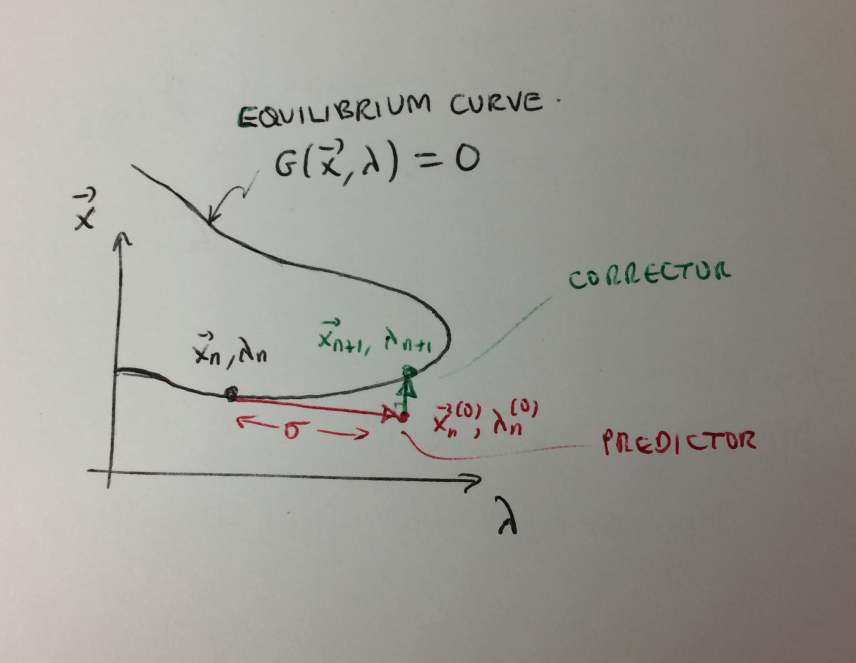
The specific algorithm I used to solve these equations was by H.B. Keller, and I took it from Appendix B of this paper. Each iteration from \(({\bf x}_n, \lambda_n)\) to \(({\bf x}_{n+1}, \lambda_{n+1})\) consists of a predictor step followed by a corrector step. The picture is as follows:

Predictor step: This is a first-order forward approximation \[ {\bf x}_n^{(0)} = {\bf x}_n + \sigma\frac{\mathrm{d}{\bf x}_n}{\mathrm{d}s}, \qquad \lambda_n^{(0)} = \lambda_n + \sigma\frac{\mathrm{d}\lambda_n}{\mathrm{d}s} \] for some small step-size \(\sigma\). We can derive the derivatives \(\mathrm{d}{\bf x}_n/\mathrm{d}s\) and \(\mathrm{d}\lambda_n/\mathrm{d}s\) at \(({\bf x}_n, \lambda_n)\) by algebraically solving equations (1) and (2). In particular, let \(J({\bf x}_n,\lambda_n) = \partial{\bf G}/\partial{\bf x}\) be the Jacobian matrix evaluated at \(({\bf x}_n, \lambda_n)\), and let \({\bf G}' ({\bf x}_n,\lambda_n)= \partial{\bf G}/\partial\lambda\), also evaluated at \(({\bf x}_n, \lambda_n)\). Then (2) implies that \[ \frac{\mathrm{d}{\bf x}}{\mathrm{d}s} = -J^{-1}({\bf x}_n,\lambda_n){\bf G}'({\bf x}_n,\lambda_n)\frac{\mathrm{d}\lambda_n}{\mathrm{d}s}, \] whence substituting this into (1) and rearranging gives \[ \frac{\mathrm{d}\lambda_n}{\mathrm{d}s} = \pm \left(1 + \|J^{-1}({\bf x}_n,\lambda_n){\bf G}'({\bf x}_n,\lambda_n)\|^2\right)^{-1/2}. \] The sign here determines the direction of motion along the equilibrium curve.
Corrector step: On its own, repeating the predictor iteration would lead to cumulative errors. So each time we project back on to the solution curve by solving the equations \[\begin{align*} &{\bf G}({\bf x}_{n+1}, \lambda_{n+1}) = 0, \quad (3)\\ &N({\bf x}_{n+1}, \lambda_{n+1}, \sigma) \equiv \frac{\mathrm{d}{\bf x}_n}{\mathrm{d}s}\cdot({\bf x}_{n+1} - {\bf x}_n) + \frac{\mathrm{d}\lambda_n}{\mathrm{d}s}(\lambda_{n+1}-\lambda_n) - \sigma = 0, \quad (4) \end{align*}\] The second equation here says that the projection of \(({\bf x}_{n+1}, \lambda_{n+1}) - ({\bf x}_n, \lambda_n)\) on to the tangent at \(({\bf x}_n, \lambda_n)\) has length \(\sigma\). In other words, it enforces that we step a distance \(\sigma\) along the arclength of the curve. This restriction of where we project back to the solution curve is important as it enables the algorithm to negotiate turning points in the solution curve.
Equations (3) and (4) are a system of three nonlinear equations for the unknowns \(({\bf x}_{n+1}, \lambda_{n+1}),\) and we solve them iteratively with Newton’s method, using the predictor point \(({\bf x}_n^{(0)}, \lambda^{(0)})\) as an initial guess. The convergence criterion is \(\|{\bf G}\| < \varepsilon\) for some chosen \(\varepsilon\).
In fact, there is still a problem at turning points: we need to change the sign in the first equation after passing a turning point, otherwise the solution will simply bounce back and forth around the turning point. Fortunately it is simple to identify such points by watching for a sign change of \(\mathrm{det}(\partial{\bf G}/\partial{\bf x})\).