Dynamics Notes

1.1 Definitions and constant force \(F\).

Position, velocity, acceleration. A particle is an object located at a point in space. For the time being, we will take space to be the real line \({\mathbb{R}}\), typically thought of as the \(x\)-line. The position of the particle at time \(t\) is \(x(t)\), and its velocity is \(v(t)=\dot{x}\), where the dot denotes derivative with respect to \(t\). The speed of the particle is \(|v(t)|\), and its acceleration is \(a(t)=\dot{v}=\ddot{x}\).

Example. A particle moves along the \(x\)-axis with constant acceleration \(c\). Its initial velocity (at time \(t=0\)) is \(v_0\), and its initial position is \(x_0\). What is its position at later times?

Solution. Direct integration gives \(x(t)=\tfrac{1}{2}c t^2+v_0t+x_0\). Note that either \(v_0\) or \(a\) or both could be positive, negative, or zero.

Momentum, force, and the Equation of Motion. Any particle has an associated mass \(m>0\). With velocity \(v\), its momentum is \(p=mv\). Either \(m\) or \(v\) or both could depend on time. If the particle feels a total force \(F\), then its momentum satisfies the equation of motion \(\dot{p}=F\). Unless otherwise stated, we shall always assume that \(m\) is constant; then the equation of motion (EoM) is equivalent to \(m\ddot{x}=F\). In general, \(F=F(x,\dot{x},t)\) is a function of position, velocity and time, and you may not be able to solve the EoM \(m\ddot{x}=F(x,\dot{x},t)\) explicitly; in this course, we will focus on special cases of \(F\) for which the EoM can be solved explicitly.

Vertical motion near the Earth’s surface. The acceleration due to gravity near the Earth’s surface has an approximately constant value which is traditionally denoted \(g\). The magnitude \(mg\) of the gravitational force on a falling object of mass \(m\) is called its weight. So the solution \(x(t)\) for straight up-and-down motion is the one given above, as illustrated in the example below.

Remarks. . The choice of coordinates is up to you. So you may take \(x\) to point upwards, in which case the EoM is \(m\ddot{x}=-mg\); or downwards, in which case the EoM is \(m\ddot{x}=mg\). . There are no units (meters, seconds etc), and \(g\) does not have a numerical value (whether 9.8 or anything else). . The so-called SUVAT relations have very limited applicability, and should be avoided.

Example. A projectile is shot vertically upwards with initial speed \(u\). What maximum height \(H\) does it reach? (Ignore air resistance.)

Solution. Take height to be in the positive \(x\)-direction, with the ground at \(x=0\). On the way up, we have \(x(t)=-\tfrac{1}{2}g t^2+ut\). The maximum height \(H\) occurs when \(v=0\), which is at time \(t=u/g\); so \(H=x(u/g)=u^2/(2g)\).

Exercise. A projectile is shot vertically upwards with initial speed \(u\). What is its speed \(w\) when it reaches half its maximum height, on the way up?

Sketch of solution. Half the max height is \(u^2/(4g)\), and \(x(t)\) equals this when \[t=t_1=(u/g)(1-1/\sqrt{2}).\] So the speed \(w\) at half max height is \[w=u-gt_1=u/\sqrt{2}.\]

1.2 The cases \(F=F(t)\) and \(F=F(v)\).

Previously we dealt with the easy case where the force \(F\) is constant. The cases \(F=F(t)\) and \(F=F(v)\) are also straightforward in principle, meaning that you can solve them as long as you can do the integrals that crop up. The case \(F=F(t)\) gives the equation of motion \(m\ddot{x}=F(t)\), which is solved by direct integration. The case \(F=F(v)\) gives the equation of motion \(m\dot{v}=F(v)\); this can be solved by separation of variables to get \(v(t)\), which is then integrated with respect to \(t\) to get \(x(t)\).

Example. Here \(F=F(t)\). A particle of mass \(m=1\) lies at rest at \(x=0\). A force field is switched on at time \(t=0\) and exerts a force \(F(t)={\rm e}^{-t}\). Find the subsequent position \(x(t)\) of the particle.

Solution. The equation of motion is \(\dot{v}={\rm e}^{-t}\), so \[v(t)=\int {\rm e}^{-t}\,dt =1- {\rm e}^{-t},\] using \(v(0)=0\). Now integrate again to get \[x(t)=t+{\rm e}^{-t}-1,\] using \(x(0)=0\). Note that for large \(t\), the force dies away, so we expect the particle to just drift with constant velocity; from our solution we see that this is indeed what happens. (Exercise in analysis: prove that \(x(t)>0\) for all \(t>0\), as must be the case physically.)

Example. Here \(F=F(v)\). A bead of mass \(m\) slides along a horizontal straight wire, slowed by a frictional force of magnitude \(b\exp(av)\), where \(a\) and \(b\) are constants. If its initial speed is \(u\), how long does it take to come to rest?

Solution. Here \(m\dot{v}=-b\exp(av)\), which is a separable first-order ODE. You can find the general solution of this, and then put in the initial condition. Another way is to do both at the same time, namely as follows: \[\int_u^0 e^{-av}\,dv = -\frac{b}{m} \int_0^T dt,\] which gives \(T=m\{1-\exp(-au)\}/(ab)\). Note that \(b>0\), and \(T>0\) whatever the sign of \(a\).

Example. A parachutist of mass \(m\), starting from rest at time \(t=0\), drifts downwards. The force due to air resistance has magnitude \(b|v|\), where \(b\) is a constant. Derive an expression for her speed \(w(t)=|v(t)|\). What is the ‘least upper bound’ of this speed?

Solution. Let us take \(x\) to point downwards, so that \(v>0\) and hence \(w=v\). The equation of motion is \(m\dot{w}=mg-bw\) with initial condition \(w(0)=0\). We can integrate this either by linearity, or by separating variables. (Exercise: do it both ways.) Separating variables gives \[\int_0^t dt = \int_0^w \frac{dv}{g-bv/m} = -\frac{m}{b}\left[\log\left(g-\frac{bv}{m}\right)\right]_0^w = -\frac{m}{b}\log\left(\frac{g-bw/m}{g}\right).\] This then gives \[w(t)=\frac{mg}{b}\left[1-\exp\left(-\frac{bt}{m}\right)\right].\] The terminal speed is \(w(\infty)=mg/b\), and \(w\) approaches this value asymptotically.

Exercise. A unit mass (\(m=1\)) moving along the \(x\)-axis with velocity \(v\) is subject to a force \(F=2\sqrt{v}\). Given that \(x(0)=0=v(0)\), find \(x(t)\).

Sketch of solution. From \(dv/dt=2\sqrt{v}\) we get \(v(t)=t^2\). Integrating this gives \[x(t)=\tfrac{1}{3}t^3.\]

1.3 The case \(F=F(x)\).

To solve \(m\ddot{x}=F(x)\), we can use a trick. Think of \(v\) being a function of \(x\). Then \[F(x)=m\frac{d}{dt}v(x(t))=m\frac{dv}{dx}\frac{dx}{dt}=m\frac{dv}{dx}v,\] by the Chain Rule, and so \[m\frac{dv}{dx}v = F(x),\] which is a first-order separable ODE. Integrating it gives \[\tfrac{1}{2}m v^2=\int F(x) \,dx,\] and hence you get \(v(x)\).

Example. A particle of mass \(m=2\) can glide smoothly along the \(x\)-axis. If it is subject to a force \(F=3x^2\), and \(x=1=v\) at \(t=0\), find how long it takes for the particle to reach \(x=9\).

Solution. From \(3x^2=2v\,dv/dx\) we get \(v^2=x^3\). Since we expect \(v>0\) (force and initial \(v\) are both positive), we get \(v=dx/dt=x^{3/2}\). Integrating this gives \[\int_1^9 x^{-3/2}\,dx=\int_0^Tdt \quad\Rightarrow\quad T=4/3.\]

Example. A unit-mass particle travels along the \(x\)-axis from \(x=-\infty\) to \(x=\infty\), subject to a force \(F(x)=1/(1+x^2)\). If its velocity as \(x\to-\infty\) is \(u_0\), what is its velocity \(u_1\) as \(x\to\infty\)?

Solution. Note \(F>0\) so velocity will increase: the particle gets a ‘positive kick’ as it passes \(x=0\). From \(v\,dv/dx=1/(1+x^2)\) we get \[\int_{u_0}^{u_1}v\,dv = \int_{-\infty}^{\infty}\frac{dx}{1+x^2},\] giving \(u_1=\sqrt{u_0^2+2\pi}\).

Remark. For problems with \(F=F(v)\) we can use \(F(v)=m\,dv/dt\) as we saw before. But it may sometimes be more convenient to use \(F(v)=mv\,dv/dx\), in situations where we want \(v(x)\) rather than \(v(t)\). See the following exercise.

Exercise. Find \(v(x)\) if \(m=1\), the force is \(F=-v^2\), and \(v=1\) when \(x=0\).

Sketch of solution. From \(v\,dv/dx=-v^2\) we get \(v(x)=\exp(-x)\).

1.4 Two more general examples.

‘Mixed’ example. A unit mass moves along a line, acted on by a force \(F(v,t)=-v+\exp(-t)\), where \(v\) is its velocity. Given that \(v(0)=0\), find \(v(t)\).

Solution. The equation of motion is \[\dot{v}=-v+e^{-t},\] which is a linear ODE for \(v(t)\). Solving it via an integrating factor \(\exp(t)\) gives \[v(t)=t e^{-t}.\]

Rocket: non-constant mass. A rocket of mass \(m(t)\) burns fuel at a constant rate \(\dot{m}=-c\), where \(c>0\). This produces a constant thrust \(F=k|\dot{m}|=kc\). The rocket starts at rest at \(x=0\), with initial mass \(m_0\). Find its subsequent position \(x(t)\).

Solution. The constant force gives \(mv=kct\). Now \(m(t)=m_0-ct\), so \[v(t)=\frac{kct}{m_0-ct}=-k+\frac{km_0}{m_0-ct}\] for \(0\leq t<m_0/c\). Integrating this gives \[x(t)=-kt+\frac{km_0}{c}\log\left(\frac{m_0}{m_0-ct}\right)\] for \(0\leq t<m_0/c\). Note that for small \(t\) we have \[v(t)\approx\frac{kct}{m_0};\] whereas when \(t\to m_0/c\) we get \(v\to\infty\) and \(x\to\infty\). The latter is rather unphysical, since the rocket would have to burn itself up completely.

Exercise. Consider a particle of mass \(m=2\) subject to a force \(F=F(t,v)=t-v\). If at \(t=0\) the particle is at \(x=0\) and at rest, find \(x(t)\).

Sketch of Solution. The equation of motion is \(2\,dv/dt = t-v\). This is linear in \(v\), so can be solved with an integrating factor \(I=\exp(t/2)\), giving (after integration by parts) \[v(t) = t + 2\exp(-t/2) -2.\] This is then easily integrated further to give \[x(t) = \tfrac{1}{2}t^2 -2t - 4\exp(-t/2) +4.\]

Further reading: Gregory section 4.1.

2.1 Energy.

Definitions. Consider the case \(F=F(x)\), and write \(V(x)=-\int F(x)\,dx\). Then \[\frac{d}{dx}\left(\tfrac{1}{2}mv^2\right)=mv\frac{dv}{dx}=ma=F=-\frac{dV}{dx},\] and so \[E=\tfrac{1}{2}mv^2 + V(x)\] is constant in time, since the chain rule gives \[\frac{dE}{dt} = \frac{dE}{dx} \dot{x} = 0.\] This quantity \(E\) is the energy of the particle, and we say that it is conserved. The term \(\tfrac{1}{2}mv^2\) is the kinetic energy, and \(V(x)\) is the potential energy; neither of these is conserved in general.

Remarks. (i) A force of the form \(F(x)\) is said to be conservative, since it conserves energy. (ii) The potential \(V\), and hence the energy \(E\), are only defined up to an arbitrary constant. (iii) The simplest example is where \(F\) is constant, so \(V\) is linear in \(x\). Gravity near the Earth’s surface is of this type: measuring \(x\) upwards, we have \(F=-mg\) and so \(V=mgx\). (iv) Using conservation of energy can give us a good picture of the particle’s motion, even when we cannot get \(x(t)\) explicitly. The example in 2.2 illustrates this. (v) The energy \(E\) is constant for a given solution; a different solution will, in general, have a different energy.

Example. Falling under gravity. Here \(E=\tfrac{1}{2}mv^2+mgx\), with \(x\) being measured upwards. For the solution determined by \(v=1=x\) at \(t=0\), we get \(E=m/2+mg\) for all \(t\).

Exercise. A unit-mass particle (\(m=1\)) moves along the \(x\)-axis, subject to a force \(F=-2x^3\). Derive an expression for its energy \(E\), such that \(E=0\) if the particle is stationary at \(x=0\). Then compute \(E\) if its speed is \(v=1\) at \(x=1\).

Sketch of solution. \(E=\tfrac{1}{2}(v^2 + x^4)\), and \(E=1\) in this case.

2.2 Motion in a potential.

Consider a particle moving along the \(x\)-axis, in a potential \(V(x)\). Except in simple cases, we won’t know exactly what the trajectory \(x(t)\) is. But we can say something about what it looks like, just by using the fact that the energy \(E\) is constant. It is valid (although just an analogy) to picture the particle as a ball rolling on the graph of \(V\), with gravity acting downwards.

Example. A double-well potential. A particle of mass \(3\) moves in a potential \[V(x) = \frac{x^4}{4}-\frac{x^3}{3}-x^2.\] Find the force \(F\). At what points can the particle remain at rest (be in equilibrium)? Describe the motion of the particle if \(x(0)=2\) and \(v(0)=1\). How do things differ if instead \(x(0)=2\) and \(v(0)=-2\)?

Remark. The equation of motion is equivalent to \(\tfrac{1}{2}m \dot{x}^2+V(x)=E\), which is separable. The resulting integral could be done, to obtain \(x(t)\), but it’s messy.

Solution. The force is \[F(x)=-\frac{dV}{dx}=-x^3+x^2+2x=-x(x-2)(x+1),\] so there are three equilibria, namely at \(x=-1,0,2\). The potential \(V(x)\) is a ‘double well’, with a local maximum at \(x=0\), and local minima at \(x=-1\) and \(x=2\). Note that \(V(0)=0\) and \(V(-1)=-5/12 > V(2)=-8/3\). The energy \(E\) is constant, and satisfies \[E - V(x) = \tfrac{1}{2}mv^2 \geq0,\] which restricts \(x\).

First consider the case \(x(0)=2\) and \(v(0)=1\). So the particle starts at the bottom of the right-hand well. For it ever to get over the ‘hill’ at \(x=0\), its energy would have to be greater than \(V(0)=0\). But in this case, the initial conditions give \(E=-7/6\), and so the particle cannot get over the hill: it does not have enough energy to do so, and just oscillates back and forth about \(x=2\), without ever reaching \(x=0\).

Next take the case \(x(0)=2\) and \(v(0)=-2\): here \(E=10/3\), so the particle gets over the hill, and passes \(x=-1\) before reaching a minimum value of \(x\) and turning back; in other words, it continues to visit all the equilibrium points, back and forth.

Question. Starting at \(x=1\) with speed \(u\), how big does \(u\) have to be to reach \(x=-1\)? Answer: we need enough initial kinetic energy to get over the hill at \(x=0\). Using \(V(1)=-13/12\) then gives \(u>\sqrt{13/18}\).

Exercise. In the example above, suppose that the particle starts at \(x=-1\), with a positive initial velocity \(v\). How large does \(v\) have to be to ensure that the particle reaches \(x=1\)?

Sketch of solution. To get over the hill at \(x=0\), we need \[\frac{3}{2} v^2 + V(-1) > V(0).\] This gives \(v > \sqrt{5/18}\).

2.3 The simple harmonic oscillator.

For a springy or elastic force, the simplest approximation is Hooke’s Law. This says that if you extend or compress a spring by a distance \(x\), then the restoring force is \(F=-kx\), where \(k>0\) is the spring constant. This force is conservative, with potential energy \(V(x)=-\int F=\tfrac{1}{2}kx^2\), so \(x=0\) is an equilibrium position. The equation of motion is \(m\ddot{x}=-kx\); and the general solution of this is \[x(t)=A\cos(\omega t)+B\sin(\omega t),\] where \(\omega=\sqrt{k/m}\) is the angular frequency of the oscillation. This is simple harmonic motion: it is periodic in \(t\) with period \(T=2\pi/\omega=2\pi\sqrt{m/k}\). The amplitude of the oscillation is \(C=\sqrt{A^2+B^2}\).

We could add gravity: think of the spring hanging downwards. If \(x\) is taken to point up, the equation of motion becomes \(m\ddot{x}=-kx-mg\). Then the solution \(x(t)\) is as before, with the constant \(-mg/k\) added to it (a particular integral). The effect of gravity is simply to shift the equilibrium position from \(x=0\) to \(x=-mg/k\).

Exercise. A mass \(m=2\) is attached to a spring with spring constant \(k=8\). The equilibrium position is \(x=0\). What is the position \(x(t)\) of the mass if the initial conditions are \(x(0)=2\) and \(\dot{x}(0)=-2\)? What are the period \(P\) and the amplitude \(S\) of the oscillation?

Sketch of solution. The angular frequency is \(\omega=2\), and the solution is \[x(t)=2\cos(2t)-\sin(2t).\] Also \(P=\pi\) and \(S=\sqrt{5}\).

2.4 Damped oscillators.

Consider the suspension of a car, say one of the front wheels supporting a mass \(m\). It has a spring, with spring constant \(k\). The only effect of gravity is to compress the spring so that it has a new natural length, and we ignore gravity in what follows. Without damping, the height deviation \(x(t)\) of the car from its equilibrium height satisfies \(m\ddot{x}=-kx\), and we get simple harmonic motion as previously.

Now add damping (a shock absorber) by putting in a force proportional to \(-\dot{x}\); for convenience, take this to be \(-2mb\dot{x}\). Here \(2mb>0\) is the damping constant. Our equation of motion is now \[m\ddot{x}=-kx-2mb\dot{x} \implies \ddot{x}+2b\dot{x}+\omega^2 x=0,\] with \(\omega=\sqrt{k/m}\) as before. The auxiliary equation for this ODE is \(\lambda^2+2b\lambda+\omega^2=0\), with roots \(\lambda_{\pm}=-b\pm\sqrt{b^2-\omega^2}\). There are three characteristic cases.

\(\bullet\) The first, if \(b>\omega\), is overdamping. Here the \(\lambda_{\pm}\) are real and negative, and so \[x(t)=A_+\exp(\lambda_+t)+A_-\exp(\lambda_-t)\] is exponentially decaying. There is no oscillation as such.

\(\bullet\) The second type, if \(0\leq b<\omega\), is underdamping. Here the \(\lambda_{\pm}\) are complex, in fact \(\lambda_{\pm}=-b\pm iq\) where \(q^2=\omega^2-b^2\). The solution now is \[x(t)=e^{-bt}[A\cos(qt)+B\sin(qt)].\] There are oscillations, but their amplitude decays exponentially with time. A car suspension is slightly underdamped, if it’s working properly.

\(\bullet\) The third type, if \(b=\omega\), is critical damping. The solution now is \[x(t)=e^{-bt}(A+Bt).\] The behaviour is then rather similar to the overdamped case.

Exercise. The deformation \(u(t)\) from equilibrium of a damped spring is described by the equation \(\ddot{u}+2\dot{u}+2u=0\). Given that the spring is initially undeformed, in other words \(u(0)=0\), and that the initial velocity is \(\dot{u}(0)=-3\), find the subsequent deformation \(u(t)\).

Sketch of solution. Auxiliary equation has roots \(\lambda=-1\pm i\), leading to \(u(t)=-3\exp(-t)\sin(t)\).

Further reading: Kibble-Berkshire sections 2.1, 2.2, 2.5; Gregory sections 5.1–5.3.

3.1 Forcing and resonance.

Say our car is travelling on a corrugated road surface. This is modelled by adding a forcing term on the right-hand-side, such as \(C\sin(pt)\). Let us first look at a simple example with no damping, namely \[m\ddot{x}+kx=m\sin(pt).\] The general solution (CF plus PI) is, with \(\omega=\sqrt{k/m}\) as before, \[x(t) = A\cos(\omega t)+B\sin(\omega t)+\frac{\sin(pt)}{\omega^2-p^2},\] provided \(|p|\neq\omega\). We have a mixture of two oscillations with angular frequencies \(\omega\) and \(p\). Note that \(x(t)\) is bounded. But if \(p=\omega\), then the solution is \[x(t) = A\cos(\omega t)+B\sin(\omega t)-\frac{t\cos(\omega t)}{2\omega}, % x(t) = A\cos(t)+B\sin(t)-\half t \cos(t),\] and the amplitude grows without bound as \(t\) increases. This is resonance: the applied force is synchronized with the natural oscillation of the mass-spring system.

Now put in damping. For example, consider the system \[\ddot{x}+3\dot{x}+2 x=\sin(pt),\] The CF is as in section 2.4 (overdamped), a combination of \(e^{-t}\) and \(e^{-2t}\), and \(x_{CF}\to0\) as \(t\to\infty\): it is a transient response. By contrast, the steady-state response is a periodic particular integral \(x_{PI}\), of the form \(x(t)=A\cos(pt)+B\sin(pt)\). Defining \(\phi\) by \(\tan(\phi)=2bp/(\omega^2-p^2)\), \(x_{PI}\) can be written in the form \(x_{PI}(t)=C\sin(pt-\phi)\). With damping, there is no resonance, for any value of \(p\). The phase difference \(\phi\) between forcing and response is due to a lag between when the car feels an upwards force from the uneven road, and when it actually moves up.

Exercise. The behaviour \(x(t)\) of a forced damped system is described by the equation \(\ddot{x}+4\dot{x}+x-\sin(t)=0\). Find the steady-state response \(x_S(t)\) of this system, and compute the phase difference between it and the external force.

Sketch of solution. The steady-state response is a periodic particular integral of the differential equation, and this is \[x_S(t) = -\tfrac{1}{4}\cos(t).\] The phase difference between this and \(\sin(t)\) is \(\pi/2\).

3.2 Small Oscillations.

Motion near stable equilibria. A conservative force \(F(x)=-V'(x)\) has an equilibrium at \(x=x_0\) if \(F(x_0)=0\). A particle can sit at \(x=x_0\), at rest. The equilibrium is stable if \(x_0\) gives a local minimum of \(V\), so \(V''(x_0)>0\). If, on the other hand, \(V''(x_0)\leq0\), then the equilibrium is unstable. If you graph \(V(x)\), then you can imagine a particle rolling on it, with gravity acting downwards (but note that this is just an analogy). For example, \(V(x)=x^4-2x^2\) has \(V'(x)=4x(x+1)(x-1)\), so there is an unstable equilibrium at \(x=0\) and stable equilibria at \(x=\pm1\). For a stable equilibrium, if you perturb the particle by a small amount, it will stay close to the equilibrium, oscillating around it.

Simplest case. The simplest case is \(V(x)=\tfrac{1}{2}k x^2\), with \(k>0\) (the simple harmonic oscillator). There is a stable equilibrium at \(x=0\). Then \(m\ddot{x}=-kx\), and the system oscillates with angular frequency \(\omega=\sqrt{V''(0)/m}=\sqrt{k/m}\). The period is \(2\pi/\omega=2\pi\sqrt{m/k}\).

General potential. Suppose that \(V(x)\) has a local minimum at \(x_0\). Write \(x(t)=x_0+\epsilon(t)\) where \(\epsilon(t)\) is small. The equation of motion is \[m\ddot{\epsilon}=F(x_0+\epsilon)=F'(x_0)\epsilon+\ldots=-V''(x_0)\epsilon+\ldots,\] using the Taylor series (the dots denote terms like \(\epsilon^2\), much smaller than \(\epsilon\)). Thus we get approximate simple harmonic motion, with angular frequency approximately \(\omega=\sqrt{V''(x_0)/m}\) and period \(2\pi/\omega\). Note that \(\epsilon\) remains small, so this makes sense. In effect, we are approximating the graph of \(V(x)\) by a parabola near \(x_0\).

Example. Return to the example of 2.2, namely \(m=3\) and \[V(x)=\frac{x^4}{4}-\frac{x^3}{3}-x^2.\] There are equilibria at \(x=-1\) and \(x=2\). A particle at rest at \(x=-1\), perturbed slightly, will oscillate about \(x=-1\) with approximate angular frequency \(\omega=\sqrt{V''(-1)/m}=\sqrt{3/3}=1\) and period \(2\pi\).

Exercise. For this system, compute the period \(P\) of small oscillations about \(x=2\).

Sketch of solution. The approximate angular frequency is \(\omega=\sqrt{V''(2)/m}=\sqrt{6/3}=\sqrt{2}\), so the period is \(P=\pi\sqrt{2}\).

3.3 Momentum and Collisions 1.

Conservation of momentum. If there are no external forces, and \(N\) particles with momenta \(p_1,p_2,\ldots,p_N\), then the total momentum \[p=p_1+p_2+\ldots+p_N\] is conserved, and does not change when the particles collide. By contrast, the total energy (just kinetic energy, since there are no external forces), namely \[E=\tfrac{1}{2}m_1v_1^2+\tfrac{1}{2}m_2v_2^2+\ldots+\tfrac{1}{2}m_Nv_N^2,\] need not be conserved. A collision which does conserve \(E\) is said to be elastic; but otherwise the collision is inelastic. For example, the collision of two billiard balls is (almost) elastic, whereas the collision of two lumps of soft dough is inelastic.

Example 1. A particle of mass \(2m\) and speed \(v\) collides head-on with a particle of mass \(m\) at rest. The two then continue to move in the same direction, with the heavier particle moving at speed \(v/2\). What is the speed \(u\) of the lighter particle, and what fraction of the initial energy is lost in the collision?

Solution. Conservation of momentum says that \(2mv+m.0=2mv/2+mu\), and so \(u=v\). The initial energy is \(E_i=\tfrac{1}{2}(2m)v^2=mv^2\), and the final energy is \(E_f=\tfrac{1}{2}(2m)(v/2)^2+\tfrac{1}{2}mv^2=3mv^2/4\). So the fraction of energy lost is \((E_i-E_f)/E_i=1/4\).

Exercise. A particle of mass \(2m\) and speed \(v\) collides head-on with a particle of mass \(m\) at rest. The two then continue to move in the same direction, with the lighter particle moving at speed \(2v/3\). What is the speed \(u\) of the heavier particle, and what fraction of the initial energy is lost in the collision?

Sketch of solution. Conservation of momentum gives \(u=2v/3\). The final energy is \(E_f=2mv^2/3\). So the fraction of energy lost is \((E_i-E_f)/E_i=1/3\). Remark. In effect, the two particles have coalesced.

3.4 Momentum and Collisions 2.

Example 2. A particle of mass \(2m\) and speed \(v\) collides elastically with a particle of mass \(m\) at rest. Afterwards, both move in the same direction. What is the speed of each particle after the collision?

Remark. Note that instead of being given one of the speeds after the collision, as in example 1, we are instead told that the collision is elastic.

Solution. Let \(w\) be the speed of the heavy particle, and \(u\) the speed of the light particle, after the collision. Conservation of momentum gives \(2mv=2mw+mu\) and so \(w=v-u/2\). Conservation of energy (elastic) says \(mv^2=mw^2+mu^2/2\). Eliminating \(w\) gives \(vu=3u^2/4\). Now \(u=0\) is not the desired solution (this is when the two particles miss each other), so \(v=3u/4\). Thus \(u=4v/3\) and \(w=v/3\).

Example 3. Two particles with masses 1 and 2 respectively each move with speed \(v\), towards each other, on the \(x\)-axis. After colliding they remain on the \(x\)-axis, with velocities \(v_1\) and \(v_2\) respectively. Given that \(v\) is fixed, what are \(v_1\) and \(v_2\) if the loss of energy is as great as it can be?

Solution. Let us say that particle 1 is moving leftwards and particle 2 rightwards (this is to establish signs). The conservation of momentum equation is \(2v-v=2v_2+v_1\), and so \(v_1=v-2v_2\). Now the loss of energy is \[E_{\rm loss} = (\tfrac{1}{2}\times2\times v^2+\tfrac{1}{2}\times v^2) - (\tfrac{1}{2}\times2\times v_2^2+\tfrac{1}{2}\times v_1^2) = v^2+2vv_2-3v_2^2,\] where we have used conservation of momentum to eliminate \(v_1\). Now energy loss is maximized when \(dE_{\rm loss}/dv_2=0\) which gives \(v_2=v/3\), and hence \(v_1=v-2v_2=v/3\).

Exercise. Describe what actually happens in this maximal-energy-loss situation: what is the ‘after’ picture? What fraction of energy is lost?

Sketch of solution. Since \(v_2=v_1\), the two particles have coalesced. The initial energy is \((3/2)v^2\), and \(E_{\rm loss} = (4/3)v^2\), so \(8/9\) of the energy is lost.

Further reading: Kibble-Berkshire sections 2.2, 2.6, 2.9; Gregory sections 5.4, 6.3, 10.6.

4.1 Velocity and relative motion.

Position & frames of reference. A particle is an object with a mass \(m\), located at a point in 3-dimensional space. Its position is described by a position vector \({\bf r}\) (relative to some origin \({\bf O}\)). We can use Cartesian coordinates \((x,y,z)\) by letting \({\bf i}\), \({\bf j}\) and \({\bf k}\) be the unit vectors along the \(x\)-, \(y\)- and \(z\)-axes respectively (the usual Cartesian axes), and writing \({\bf r}=x{\bf i}+y{\bf j}+z{\bf k}\). This system of axes is an example of a frame of reference. For motion in a plane, use \({\bf r}=x{\bf i}+y{\bf j}\).

Remark. You must always distinguish carefully between vectors and numbers: underline vectors, and do not underline numbers. In printed material, vectors are boldface.

Velocity & acceleration. The trajectory of a particle is given by \({\bf r}(t)=x(t){\bf i}+y(t){\bf j}+z(t){\bf k}\). Its velocity is \({\bf v}=\dot{\bf r}\), where as usual the dot denotes derivative with respect to time \(t\). If \({\bf r}=x{\bf i}+y{\bf j}+z{\bf k}\), then \({\bf v}=\dot{x}{\bf i}+\dot{y}{\bf j}+\dot{z}{\bf k}\). The speed of the particle \(v=|{\bf v}|\) is a real number with \(v\geq0\). The acceleration is \({\bf a}=\dot{\bf v}=\ddot{\bf r}\).

Examples. (a) If \({\bf r}=t{\bf i}+{\bf j}+t^2{\bf k}\), then \({\bf v}={\bf i}+2t{\bf k}\), \(v=\sqrt{1+4t^2}\) and \({\bf a}=2{\bf k}\). (b) If \({\bf a}=2{\bf k}\) with \({\bf v}(0)={\bf i}\) and \({\bf r}(0)={\bf j}+{\bf k}\), then \({\bf r}(t)=t{\bf i}+{\bf j}+(t^2+1){\bf k}\).

Momentum, force, equation of motion. The momentum of a particle with mass \(m\) and velocity \({\bf v}\) is the vector \({\bf p}=m{\bf v}\). If an external force \({\bf F}\) acts on the particle, then its equation of motion is \(\dot{{\bf p}}={\bf F}\). If \(m\) is constant (which we assume unless otherwise stated), this is equivalent to \(m\ddot{{\bf r}}={\bf F}\).

Relative motion. If particles \(A\) and \(B\) are located at \({\bf r}_A\) and \({\bf r}_B\) respectively, then the position of \(B\) relative to \(A\) is \({\bf r}_B-{\bf r}_A\). If they are moving with velocities \({\bf v}_A\) and \({\bf v}_B\) respectively, then the velocity of \(B\) relative to \(A\) is \({\bf v}_B-{\bf v}_A\).

Example. Two particles have positions \({\bf r}_A=2t{\bf i}+{\bf j}+t^2{\bf k}\) and \({\bf r}_B=-t{\bf i}\) respectively. Then the relative velocity of \(B\) with respect to \(A\) is \({\bf v}_{rel}= {\bf v}_B-{\bf v}_A=-{\bf i}-(2{\bf i}+2t{\bf k})=-3{\bf i}-2t{\bf k}\).

Exercise. Bob is going north (direction \({\bf j}\)) with speed 10, and feels a headwind of speed 25. What is the wind velocity relative to the ground? If Bob now goes east (direction \({\bf i}\)) at speed 15, what wind does he feel?

Solution. Let \({\bf v}_B\) denote Bob’s velocity and \({\bf v}_w\) the wind velocity, both relative to the ground. For the first part, we have \({\bf v}_B=10{\bf j}\) and \({\bf v}_w-{\bf v}_B=-25{\bf j}\). Thus \({\bf v}_w=-15{\bf j}\) (ie southward at speed 25). For the second part, we have \({\bf v}_B=15{\bf i}\) and \({\bf v}_w=-15{\bf j}\), so \({\bf v}_w-{\bf v}_B=-15{\bf j}-15{\bf i}\): Bob feels a wind of speed \(15\sqrt{2}\) in the direction \(-({\bf i}+{\bf j})/\sqrt{2}\).

4.2 Sliding down an inclined plane.

A mass \(m\) is free to slide down a plane which is inclined at an angle \(\alpha\) to the horizontal. Gravity acts downwards, and there is a frictional force (directed up the slope) with magnitude \(\mu N\), where \(\mu\) is a positive constant, and \({\bf N}\) is the normal force exerted by the inclined plane on the particle. (The direction of \({\bf N}\) is perpendicular to the plane.) Starting from rest, how far does the particle travel in time \(t\)? How large does \(\alpha\) have to be for the mass to move at all?

Solution. Let us take \({\bf i}\) (and the \(x\)-axis) to point down the slope. Take \({\bf j}\) to be perpendicular to \({\bf i}\) and the slope, pointing outwards. Motion is in the \(x\)-direction. The weight of the particle is downwards, with magnitude \(mg\). Its component in the \({\bf j}\)-direction is \(-mg\cos\alpha\), and so \({\bf N}=mg(\cos\alpha){\bf j}\) (there is no net force in the \({\bf j}\)-direction). Hence the total force in the \(x\)-direction is \[F=-\mu mg\cos\alpha+mg\sin\alpha,\] which is constant; so \[x(t)=\tfrac{1}{2}g(\sin\alpha-\mu\cos\alpha)t^2,\] provided \(\tan\alpha>\mu\). If \(\tan\alpha\leq\mu\), then the particle does not move (the friction is too great), and \(x(t)=0\) for all \(t\).

Exercise. You are free to choose a different basis and coordinates, and this does not affect the answer. Write out an alternative solution, taking \({\bf i}\) to be horizontal and \({\bf j}\) to be upwards.

Sketch of solution. The downwards slope is in the direction given by the unit vector \({\bf c}={\bf i}\cos\alpha-{\bf j}\sin\alpha\). The total force acting on the mass is \[{\bf F}= -mg{\bf j}+ N({\bf i}\sin\alpha+{\bf j}\cos\alpha)-\mu N{\bf c}.\] Now \({\bf F}\) has to be in the \({\bf c}\)-direction, and this gives \(N=mg\cos\alpha\). Then \[{\bf F}= mg(\sin\alpha-\mu\cos\alpha){\bf c},\] and the distance travelled in time \(t\) is \(\tfrac{1}{2}g(\sin\alpha-\mu\cos\alpha)t^2\).

4.3 Motion in an electromagnetic field.

A particle with mass \(m\) and electric charge \(q\), placed in an electric field \({\bf E}\) and a magnetic field \({\bf B}\), feels the Lorentz force \[{\bf F}= q({\bf E}+{\bf v}\times{\bf B}).\] In general, \({\bf E}\) and \({\bf B}\) can vary in space and time, but we shall take them to be constant

Vector product. Recall that \({\bf i}\times{\bf j}={\bf k}\), \({\bf j}\times{\bf i}=-{\bf k}\), \({\bf j}\times{\bf k}={\bf i}\) etc, cyclic in \(ijk\).

Example. Take \({\bf E}={\bf 0}\) and \({\bf B}=B{\bf k}\) with \(B\) constant, and with initial conditions \({\bf r}(0)={\bf 0}\) and \(\dot{{\bf r}}(0)=u{\bf i}\). The equation of motion is \[m\ddot{x}{\bf i}+m\ddot{y}{\bf j}+m\ddot{z}{\bf k}=qB\dot{y}{\bf i}-qB\dot{x}{\bf j},\] which is a coupled system of equations for \((x,y,z)\). In this case, the equation for \(z\) decouples, and we just get \(z(t)=0\) for all \(t\). The \(x,y\) equations can be integrated once, and using the initial conditions we get \[m\dot{x}=qBy+mu, \quad m\dot{y}=-qBx.\] Eliminating \(y\) from these gives \(\ddot{x}=-\omega^2 x\), where \(\omega=qB/m\). This is simple harmonic motion: the solution for \(x\) is \[x(t)=\frac{u}{\omega}\sin(\omega t),\] and then \(y\) is \[y(t)=\frac{u}{\omega}(\cos(\omega t)-1).\] Notice that \(x^2+(y+p)^2=p^2\), where \(p=u/\omega\). Thus the motion is on a circle in the \((x,y)\)-plane, with radius \(p=um/(qB)\) and angular frequency \(\omega=qB/m\). This is called cyclotron motion.

Exercise. A particle of mass \(m\) and charge \(q\) moves in an electromagnetic field \({\bf E}=E{\bf k}\) and \({\bf B}=B{\bf k}\), where \(E\) and \(B\) are constant. Find its position \({\bf r}(t)\), given the initial conditions \({\bf r}(0)={\bf 0}\) and \(\dot{{\bf r}}(0)=u{\bf i}\).

Sketch of solution. The \(xy\) equations, and hence the \(xy\)-behaviour, are exactly as in the given example. The \(z\) equation is \(m\ddot{z}=qE\), with solution \(z(t)=qEt^2/(2m)\).

4.4 Conservative forces and potential energy.

Energy. The kinetic energy of a particle of mass \(m\) and speed \(v\) is \(\tfrac{1}{2}mv^2\). If the force \({\bf F}\) depends only on position \({\bf r}\), and if there exists a real function \(V({\bf r})\) such that \[{\bf F}=\left( -\frac{\partial V}{\partial x}, -\frac{\partial V}{\partial y}, -\frac{\partial V}{\partial z} \right) = -\frac{\partial V}{\partial x}{\bf i}-\frac{\partial V}{\partial y}{\bf j}-\frac{\partial V}{\partial z}{\bf k},\] then the force is conservative, and \(V\) is called the potential energy. The total energy is \[E({\bf r},{\bf v})=\tfrac{1}{2}mv^2+V({\bf r}).\]

Proposition. In a conservative force field, the total energy is conserved.

Proof. Write \({\bf v}=(v_x,v_y,v_z)\). Then \[\frac{dV}{dt} = \frac{\partial V}{\partial x}v_x+\frac{\partial V}{\partial y}v_y+ \frac{\partial V}{\partial z}v_z = -{\bf F}\cdot{\bf v},\] by the chain rule. Secondly, \[\frac{d}{dt}(\tfrac{1}{2}mv^2)=\frac{d}{dt}[\tfrac{1}{2}m(v_x^2+v_y^2+v_z^2)]= m(v_x\dot{v}_x+v_y\dot{v}_y+v_z\dot{v}_z)=m{\bf a}\cdot{\bf v}.\] And so \[\frac{dE}{dt}=(m{\bf a}-{\bf F})\cdot{\bf v}=0.\]

Remark. The force \({\bf F}=F_x{\bf i}+F_y{\bf j}+F_z{\bf k}\) is conservative if and only if \[\frac{\partial F_z}{\partial y}=\frac{\partial F_y}{\partial z}, \quad \frac{\partial F_x}{\partial z}=\frac{\partial F_z}{\partial x}, \quad \frac{\partial F_y}{\partial x}=\frac{\partial F_x}{\partial y}.\] In practice, however, it is often easier to try to find \(V\), and then \({\bf F}\) is conservative if you succeed.

Example. Take \({\bf F}=(z-y){\bf i}+(\alpha x-z){\bf j}+(\beta x-y){\bf k}\), where \(\alpha\) and \(\beta\) are constants. For which value(s) of these constants, if any, is \({\bf F}\) conservative?

Solution. If does not matter where you start; let us start with the equation \(\partial V/\partial x=y-z\). This gives \(V=(y-z)x+g(y,z)\) where \(g\) is some unknown function. Now substitute this into \(\partial V/\partial y=z-\alpha x\), which gives us \(\alpha=-1\) and \(g(y,z)=yz+h(z)\) where \(h\) is some unknown function. Finally, substitute what we have so far into \(\partial V/\partial z=y-\beta x\), which gives us \(\beta=1\) and \(h\) being constant. So the answer is that \({\bf F}\) is conservative iff \(\beta=1=-\alpha\), and the corresponding potential is \(V(x,y,z)=yx-zx+yz\) plus an arbitrary constant.

Exercise. Show that the force \({\bf F}=2xyz{\bf i}+x^2(z{\bf j}+y{\bf k})\) is conservative, and find the corresponding potential \(V\).

Sketch of solution. You could first check the equations \(\partial F_z/\partial y=\partial F_y/\partial z\) etc. But a shorter method is simply to try to find \(V\). From \(\partial V/\partial x=-2xyz\) we get \(V=-x^2yz+h(y,z)\), where \(h\) is some function of \(y\) and \(z\). Then the \(y\) and \(z\) equations say that \(h\) is in fact constant.

Further reading: Kibble-Berkshire sections 3.1, 5.2; Gregory sections 2.2, 2.6, 4.2, 6.1, 6.4.

5.1 The simple pendulum.

A point mass \(m\) is attached to one end of a rigid light rod of length \(L\). (Here ‘rigid’ means that forces along the rod cancel, and ‘light’ means that the mass of the rod can be ignored.) The rod is pivoted at the other end, and is free to swing in a vertical plane. Let \(\theta(t)\) denote the angle between the pendulum and the vertical. The gravitational potential energy is \(V=mgz\), where \(z\) is the height of the mass above its hanging-straight-down position. So \(V\) is effectively a function of \(\theta\) given by \[V(\theta)=mgL(1-\cos\theta).\] The equilibrium points are \(\theta=0\) (hanging straight down, stable) and \(\theta=\pi\) (vertically up, unstable). If the coordinate in the horizontal direction is \(x\), then \(x=L\sin\theta\), and so \[v^2=\dot{x}^2+\dot{z}^2=L^2\dot{\theta}^2.\] Here \(\dot{\theta}\) is the angular velocity; note that \(v=L|\dot{\theta}|\). The total energy, which is conserved, is \[E=\tfrac{1}{2}mL^2\dot{\theta}^2+mgL(1-\cos\theta).\] The equation of motion obtained from \(dE/dt=0\) is \(\ddot{\theta}=-(g/L)\sin\theta\). For small oscillations about the stable equilibrium, the equation becomes \(\ddot{\theta}=-g\theta/L\), and so we get simple harmonic motion with angular frequency \(\omega=\sqrt{g/L}\). But this is just an approximation for small \(\theta\).

Example. Release the pendulum from rest in a horizontal position. What is the speed \(u\) of the mass when it passes the vertical position? Solution: conservation of energy says that \(V(\pi/2)=mu^2/2+V(0)\) which gives \(u=\sqrt{2gL}\).

Exercise. If you start at \(\theta(0)=0\), with \(\dot{\theta}(0)=\omega\), how large does \(\omega\) have to be for the pendulum to ‘loop the loop’?

Sketch of solution. We need \(E=mL^2\omega^2/2>V(\pi)=2mgL\), and so \(\omega>2\sqrt{g/L}\) in order to pass \(\theta=\pi\).

5.2 Projectiles 1.

Setup. You fire a projectile at an angle \(\theta\) to the horizontal, with initial speed \(u\). The subsequent motion is in a plane. Take axes \(z\) and \({\bf k}\) upwards, and \(x\) and \({\bf i}\) horizontal, with no motion in the \(y\)-direction. The initial velocity is \[{\bf v}(0)=u{\bf i}\cos\theta+u{\bf k}\sin\theta.\] The forces are \(-mg{\bf k}\) for gravity, and \(-\lambda{\bf v}\) for air resistance. Take \({\bf r}(0)={\bf 0}\). If there is no resistance, then we get \[{\bf r}(t)=ut{\bf i}\cos\theta+(ut\sin\theta-\tfrac{1}{2}gt^2){\bf k}.\]

Example 1: time of flight and range. Suppose that the ground surface is horizontal, and that there is no resistance. Let \(T\) be the time taken for the projectile to land. In other words, \(z(T)=0\), so \[T=2ug^{-1}\sin\theta.\] Let \(X\) be the range: then \[X=x(T)=Tu\cos\theta=2u^2g^{-1}\cos\theta\sin\theta =u^2g^{-1}\sin(2\theta).\] Note that the range is maximized, for a given \(u\), by \(\theta=\pi/4\).

Exercise. What is the maximum height \(H\) of the projectile?

Sketch of solution. \(\dot{z}=0\) at time \(t=(u/g)\sin\theta\), and so \(H=(u\sin\theta)^2/(2g)\).

5.3 Projectiles 2.

Example 2: hitting a target. For a given \(u\), we want to hit a target at \((x_0,z_0)\). Is this possible, and if so what angle \(\theta\) should the projectile be shot at? Solution. Eliminate \(t\) to get the trajectory \[z(x)=x\tan\theta-\frac{gx^2}{2u^2\cos^2\theta}.\] (Note that this is a parabola.) Now \(z(x_0)=z_0\) gives an equation for \(\tan\theta\), namely (use \(\sec^2\theta=1+\tan^2\theta\)): \[p\tan^2\theta - x_0\tan\theta +(p+z_0) = 0,\] where \(p=gx_0^2/(2u^2)\). This quadratic equation for \(\tan\theta\) has a real solution iff \[x_0^2-4p(p+z_0)\geq0 \Leftrightarrow z_0\leq\frac{u^2}{2g}-\frac{gx_0^2}{2u^2}.\] If this does not hold, then the target is out of range. If it holds with \(<\), then there are two possible angles to hit the target.

Example 3. Here we include air resistance \(-\lambda{\bf v}\). Write \(\mu=\lambda/m\) and \({\bf g}=-g{\bf k}\), so that the equation of motion is \[\dot{{\bf v}}+\mu{\bf v}={\bf g}.\] This is a vector equation, but the three components are uncoupled, which makes it relatively easy. Since it is linear, we can use an integrating factor \[I=\exp\int\mu\,dt=e^{\mu t},\] and so \[{\bf v}(t)=e^{-\mu t}\int e^{\mu t}{\bf g}\,dt=\mu^{-1}{\bf g}+{\bf c}e^{-\mu t},\] where \({\bf c}\) is a constant vector. With the initial condition \({\bf v}(0)={\bf u}\) this becomes \[{\bf v}(t)=\mu^{-1}{\bf g}+e^{-\mu t}({\bf u}-\mu^{-1}{\bf g}).\] Now integrate again, with the initial condition \({\bf r}(0)={\bf 0}\), to get \[{\bf r}(t)=\mu^{-1}{\bf g}t+\mu^{-1}(1-e^{-\mu t})({\bf u}-\mu^{-1}{\bf g}).\]

Exercise. Investigate the limit \(\mu\to0\), and check that it reduces to a previous case.

Sketch of solution. Use the first three terms of the Taylor series for the exponential function, and then let \(\mu\) tend to zero. Or you can use l’Hôpital twice. You end up with \({\bf r}(t)={\bf u}t+\tfrac{1}{2}{\bf g}t^2\) as expected.

5.4 Momentum and collisions.

Momentum. A particle with mass \(m\) and velocity \({\bf v}\) has momentum \({\bf p}=m{\bf v}\). If a force \({\bf F}\) is acting, then the equation of motion is \(\dot{{\bf p}}={\bf F}\). In general, momentum is not conserved. But if (say) the \(x\)-component of the force is zero, then \(p_x\) is conserved (constant in time).

Example. Suppose that \({\bf F}\) is conservative, with potential \(V=(x+y)^2\). Then \(p_z\) and \(p_x-p_y\) are both conserved. Proof. \(\dot{p}_z=F_z=-\partial V/\partial z=0\) and \(\dot{p}_x-\dot{p}_y=F_x-F_y=-\partial V/\partial x+\partial V/\partial y=0\).

Collisions. If there are no external forces, then the total momentum is conserved. For example, one could think of particles on a frictionless horizontal table, colliding with one another. If the collision is elastic, then kinetic energy is conserved as well.

Example. A particle of unit mass is travelling with velocity \({\bf v}=3{\bf i}+3{\bf j}\) when it collides with a stationary particle of mass 2. If the unit-mass particle comes away from the collision with velocity \({\bf u}=-{\bf i}+{\bf j}\), calculate the velocity \({\bf w}\) of the other particle after the collision, and calculate the fractional loss in kinetic energy.

Solution. Total momentum before is \({\bf p}=3{\bf i}+3{\bf j}\), and total momentum after is \({\bf p}'=(-{\bf i}+{\bf j})+2{\bf w}\). Now conservation of momentum says that \({\bf p}'={\bf p}\), which gives \({\bf w}=2{\bf i}+{\bf j}\). As for the kinetic energy, before collision it was \(K=9\), and after collision it is \(K'=6\), so the fractional loss in kinetic energy is \((K'-K)/K=3/9=1/3\). (Therefore this collision was inelastic.)

Exercise. Consider two particles of equal mass. One is at rest, and is struck by the other. After the collision, the two particles are moving at right angles to each other. Prove that the collision was elastic. [Hint: if the velocities after are \({\bf u}_1\) and \({\bf u}_2\), look at \(({\bf u}_1+{\bf u}_2)\cdot({\bf u}_1+{\bf u}_2)\).]

Sketch of solution. Let \({\bf v}\) be the velocity of the moving particle before collision. Conservation of momentum says that \({\bf v}={\bf u}_1+{\bf u}_2\). Since \({\bf u}_1\cdot{\bf u}_2=0\), we get \(v^2=u_1^2+u_2^2\), and this immediately gives \(E({\rm before})=E({\rm after})\).

Further reading: Kibble-Berkshire sections 2.1, 3.2, 7.3; Gregory sections 4.4, 6.4, 10.6.

6.1 Polar basis.

Think of a planet orbiting around the sun: we may take the sun to be fixed at the origin, and the orbit to lie in a plane \({\mathbb{R}}^2\). We could use Cartesian coordinates \((x,y)\), but it is better to use polar coordinates \((r,\theta)\), where \(x=r\cos\theta\) and \(y=r\sin\theta\), and a polar basis. So \({\bf r}=r{\bf e}_r\), where \({\bf e}_r\) is the radial unit vector pointing away from the origin \({\bf O}\). The tangential unit vector \({\bf e}_\theta\) is a vector perpendicular to \({\bf e}_r\), pointing in the (anticlockwise) direction of increasing \(\theta\). All this is illustrated in the figure below. The polar-basis vectors \({\bf e}_r\) and \({\bf e}_\theta\) are unit vectors orthogonal to each other, and for a moving particle they depend on time.

Now \({\bf e}_r={\bf i}\cos\theta+{\bf j}\sin\theta\) and \({\bf e}_\theta=-{\bf i}\sin\theta+{\bf j}\cos\theta\) have time-derivatives

\[\begin{aligned} \dot{\bf e}_r &=& \frac{d\theta}{dt}\frac{d}{d\theta}{\bf e}_r =\dot{\theta}( -{\bf i}\sin(\theta) +{\bf j}\cos\theta)=\dot{\theta} {\bf e}_\theta, \\ \dot{\bf e}_\theta &=& \frac{d\theta}{dt}\frac{d}{d\theta}{\bf e}_\theta =\dot{\theta}(-{\bf i}\cos(\theta) -{\bf j}\sin\theta)=-\dot{\theta} {\bf e}_r.\end{aligned}\] Since \({\bf r}=r{\bf e}_r\), we get expressions for velocity and acceleration in this polar basis, namely \[\begin{aligned} {\bf v}&=& \dot{r}{\bf e}_r+ r\dot{\bf e}_r = \dot{r}{\bf e}_r+ r\dot{\theta} {\bf e}_\theta \mbox{ (radial component + transverse component)},\\ {\bf a}&=& \ddot{r}{\bf e}_r+ \dot{r}\dot{\bf e}_r+ \dot{r}\dot{\theta} {\bf e}_\theta +r\ddot{\theta} {\bf e}_\theta+ r\dot{\theta} \dot{\bf e}_\theta =(\ddot{r}-r\dot{\theta}^2){\bf e}_r + (2\dot{r}\dot{\theta}+r\ddot{\theta}) {\bf e}_\theta.\\\end{aligned}\]

Example. Motion in a circle at constant speed, anticlockwise. Let the circle be \(r=c\) constant. Then \({\bf v}=c\dot{\theta} {\bf e}_\theta\) and \(v=c|\dot{\theta}|\). So \(\omega=\dot{\theta}\) is constant (and positive because anticlockwise); it is called the angular velocity. Note that \(v=c\omega\), and that \({\bf r}\cdot{\bf v}=0\). The motion is described by \(\theta(t)=\omega t\). The acceleration is \({\bf a}=-c\omega^2{\bf e}_r\), so \(a=|{\bf a}|=c\omega^2\), and the acceleration is directed inwards: it is centripetal acceleration.

Exercise. For the spiral trajectory \(x=t\cos(\omega t)\), \(y=t\sin(\omega t)\), find \(r(t)\) and \(\theta(t)\), and compute the velocity \({\bf v}(t)\) in the polar basis \(\{{\bf e}_r, {\bf e}_\theta\}\).

Sketch of solution. \(r(t)=t\), \(\theta(t)=\omega t\) and \({\bf v}(t)={\bf e}_r + t\omega{\bf e}_\theta\).

6.2 Angular momentum.

A particle with position \({\bf r}\) and momentum \({\bf p}\) has angular momentum \({\bf L}={\bf r}\times{\bf p}\) about \({\bf r}={\bf 0}\). If a force \({\bf F}\) acts at the point with position vector \({\bf r}\), then its torque or moment about \({\bf r}={\bf 0}\) is \({\bf T}={\bf r}\times{\bf F}\). If the mass is constant, so that \(\dot{{\bf r}}\times{\bf p}={\bf 0}\), the equation of motion says that the rate of change of angular momentum equals the applied torque: \[\frac{d{\bf L}}{dt}={\bf r}\times\dot{{\bf p}}={\bf r}\times{\bf F}={\bf T}.\]

Proposition. Suppose that the force on a particle at position \({\bf r}\) is always proportional to \({\bf r}\). Then its angular momentum about \({\bf 0}\) is conserved.

Proof. \[\frac{d{\bf L}}{dt}=\frac{d}{dt}(m{\bf r}\times{\bf v})={\bf r}\times{\bf F}={\bf 0},\] since \({\bf F}\) and \({\bf r}\) are proportional. In other words, such a force cannot exert torque, which is what changes angular momentum.

Exercise. A particle with constant mass \(m\) has trajectory \({\bf r}(t)=t{\bf i}+{\bf j}+t^2{\bf k}\). Calculate its angular momentum \({\bf L}\) about \({\bf 0}\), and compute the torque which is affecting its motion.

Sketch of solution. \({\bf L}=m(t{\bf i}+{\bf j}+t^2{\bf k})\times({\bf i}+2t{\bf k})=m(2t{\bf i}-t^2{\bf j}-{\bf k})\). The torque is \(d{\bf L}/dt=2m({\bf i}-t{\bf j})\).

6.3 Central forces.

Definition and planar motion. A central force based at \({\bf r}={\bf 0}\) has the form \[{\bf F}=f(r)\,{\bf e}_r=r^{-1}f(r){\bf r}.\] Note that \(|{\bf F}|=|f|\). The force can act towards or away from the origin \({\bf O}\): it is attractive if \(f(r)<0\) and repulsive if \(f(r)>0\). As we saw before, the angular momentum of a particle moving in a central force is constant. Now since \({\bf L}\cdot{\bf r}(t)=0\), the motion of the particle lies in the plane through \({\bf O}\) perpendicular to the constant vector \({\bf L}\), and we take this to be the \(r\theta\)-plane. Our basis is \(\{{\bf e}_r, {\bf e}_{\theta}, {\bf k}\}\), where \({\bf k}\) is constant. The crucial point is that, because angular momentum is conserved, the plane does not change with time.

Example: gravity. Think of the Earth as being fixed at \({\bf O}\). Then the gravitational force felt by a satellite of mass \(m\) is an attractive central force, with \(f(r)=-GMm/r^2\). Here \(M\) is the mass of the Earth, and \(G=6.67\times10^{-11}\,{\rm m}^3\,{\rm kg}^{-1}{\rm s}^{-2}\) is Newton’s constant.

Exercise. Compute the acceleration \(g\) due to gravity at the surface of the Earth. The mass of the Earth is \(6\times10^{24}\,{\rm kg}\), and its radius is \(6400\,{\rm km}\).

Sketch of solution. \(|\ddot{{\bf r}}|=GM/R^2\approx9.8\,{\rm m}{\rm s}^{-2}\). (If you get \(10^6\) times this, you’ve forgotten to convert km to m.)

6.4 Motion in a central force.

Motion in polar coordinates. Take \({\bf L}\) to be in the \(z\)-direction, so that \({\bf L}=L{\bf k}\). Let \(r\) and \(\theta\) be polar coordinates in the \(xy\)-plane. Recall that \[{\bf r}=r{\bf e}_r, \quad \dot{{\bf r}}= \dot{r}{\bf e}_r+ r\dot{\theta} {\bf e}_\theta, \quad \ddot{{\bf r}}=(\ddot{r}-r\dot{\theta}^2){\bf e}_r + (2\dot{r}\dot{\theta}+r\ddot{\theta}) {\bf e}_\theta.\] Note that the angular momentum is \[{\bf L}=mr{\bf e}_r\times(\dot{r}{\bf e}_r+ r\dot{\theta} {\bf e}_\theta) = mr^2\dot{\theta}{\bf k},\] and so \(L=mr^2\dot{\theta}\). The equation of motion \(m\ddot{{\bf r}}={\bf F}\) becomes \[m(\ddot{r}-r\dot{\theta}^2)=f(r), \quad 2\dot{r}\dot{\theta}+r\ddot{\theta}=0.\] If we multiply the second of these by \(r\), we see it simply says that \(r^2\dot{\theta}\) is constant: it is equivalent to conservation of angular momentum, and we can replace it by \(mr^2\dot{\theta}=L\). Then use this to eliminate \(\dot{\theta}\) from the first (radial) equation, to leave \[m\ddot{r}-\frac{L^2}{mr^3}=f(r). \qquad\qquad(*)\] Note that the kinetic energy is \[K=\tfrac{1}{2}m|\dot{{\bf r}}|^2=\tfrac{1}{2}m(\dot{r}^2+r^2\dot{\theta}^2) =\tfrac{1}{2}m\left(\dot{r}^2+\frac{L^2}{m^2r^2}\right).\] Now any central force is conservative, and the potential energy is \[V(r)=-\int f(r)\,dr,\] where the constant of integration is usually chosen so that \(V(r)\to0\) as \(r\to\infty\). For example, the gravitational potential energy is \(V(r)=-GMm/r\). That any central force is conservative can be proved directly; but the crucial justification is that the total energy \(E=K+V\) is constant. Indeed, \[\frac{dK}{dt}=\dot{r}\left(m\ddot{r}-\frac{L^2}{mr^3}\right),\] and \(dV/dt=-f(r)\dot{r}\), so \(dE/dt=0\) is equivalent to equation (*).

Example. A unit-mass particle moves in an attractive central force of magnitude \(8/r^3\), with initial conditions \({\bf r}(0)=2{\bf e}_r\) and \(\dot{{\bf r}}(0)=3{\bf e}_r+{\bf e}_\theta\). Then we get \(L=2\), \(V(r)=-4/r^2\) so \(V=-1\) initially, \(K=5\) initially, and hence the energy is \(E=4\) for all \(t\).

Exercise. At time \(t=0\), a unit-mass particle is a distance \(D\) away from \({\bf 0}\), its velocity is at right angles to \({\bf r}\), and its speed is \(u\). What is its angular momentum \(L\) at time \(t\geq0\) and its kinetic energy \(K\) at time \(t=0\)?

Sketch of solution. We know that \(r=D\) and \(r\dot{\theta}=u\) at \(t=0\). So \(L=r^2\dot{\theta}=Du\) at \(t=0\), and therefore for all time. And at \(t=0\) we have \(K=\tfrac{1}{2}u^2\).

Further reading: Kibble-Berkshire sections 3.3–3.5, 4.1, 4.2; Gregory sections 2.2, 2.3, 4.5, 7.1, 11.2, 11.5.

7.1 Bound orbits.

We illustrate bound orbits with an example. A unit-mass particle moves under the influence of the attractive central force \(f(r)=-1/r^2\). It starts at \(r=1\), with speed \(v_0\) and direction perpendicular to \({\bf r}\). Show that the particle cannot escape to infinity (it is in a bound orbit) if \(v_0^2<2\). In this case, find the smallest and largest values of the radius \(r\). What value of \(v_0\) gives a circular orbit?

Solution. Here \(V(r)=-\int f(r)\,dr=-1/r\), and so the energy is \[E=\frac{v^2}{2}-\frac{1}{r}=\frac{v_0^2}{2}-1,\] using the initial conditions. If the particle reaches infinity we would have \(E=\tfrac{1}{2}v^2+0\geq0\), so it is bound if \(E<0\), which gives \(v_0^2<2\). For the second part, we need the angular momentum \[L=r^2\dot{\theta}=r(r\dot{\theta})=v_0.\] Expressing \(v\) in polar coordinates and eliminating \(\dot{\theta}\) then gives \[E=\frac{1}{2}\left(\dot{r}^2+\frac{v_0^2}{r^2}\right)-\frac{1}{r} =\frac{v_0^2}{2}-1.\] This equation can be written as \(\dot{r}^2+r^{-2}Q(r)=0\), where \(Q(r) = (2-v_0)^2r^2-2r+v_0^2\). The maximum and minimum values of \(r\) occur when \(\dot{r}=0\), giving a quadratic equation \(Q(r)=0\) for \(r\). The roots are \(r=r_1=1\) and \(r=r_2=v_0^2/(2-v_0^2)\). Furthermore, \(r\) is restricted to a range for which \(Q(r)\leq0\). Sketching \(Q(r)\) reveals three possibilities: if \(v_0^2<2\) then \(r\) lies between \(r_1\) and \(r_2\), a bound orbit; if \(v_0=1\) then \(r=1\) for all time, a circular orbit; if \(v_0^2>2\) then \(r_2<0\) and \(r>r_1\), an unbound trajectory. In fact, \(r_2\to\infty\) as \(v_0^2\to2\) from below: the escape speed is \(v_0=\sqrt{2}\).

Example: escape speed. This is a variant of the previous example. A projectile is launched from the surface of the Earth (radius \(R\) and mass \(M\)), with initial speed \(v_0\). How large does \(v_0\) have to be in order that the projectile escapes the Earth’s gravitational pull?

Solution. We need \[E=\tfrac{1}{2}mv_0^2-GMm/R\geq 0-0=0,\] and so \(v_0\geq\sqrt{2GM/R}\), consistent with the previous example.

Remark. The direction of the initial velocity is irrelevant. So the cheapest place for the launch is at the equator, in the direction of the Earth’s rotation: this gives a ‘slingshot’ effect. For example, the European Space Agency launch site is in South America, very close to the equator.

Exercise. A unit-mass particle is subject to an attractive central force \(f(r)=-1/r^3\). What is its escape speed \(v_0\) if it starts at \(r=R\)?

Sketch of solution. Here \(V(r)=-1/(2r^2)\), so we want \(2E=v_0^2-1/R^2\geq0\), and the escape speed is \(v_0=1/R\).

7.2 Finding the orbit.

We want to find the orbit of an object in a central force, in the form \(r=r(\theta)\). It is convenient to use the variable \(u=1/r\) rather than \(r\), so we want an equation for \(u(\theta)\). Note that the chain rule gives \[\frac{d}{dt}=\frac{Lu^2}{m}\frac{d}{d\theta}.\] This enables us to write \(\dot{r}\) and \(\ddot{r}\) as \[\dot{r}=\frac{dr}{dt}=\frac{Lu^2}{m}\frac{d}{d\theta}\left(\frac{1}{u}\right) = -\frac{L}{m}u', \quad \ddot{r}=\frac{d}{dt}\dot{r}=-\frac{L^2u^2}{m^2}u'',\] where \(u'\) denotes \(du/d\theta\) and similarly for \(u''\). Then the equation of motion (*) becomes \[u''+u=-mL^{-2}u^{-2}f(u^{-1}).\] This is the orbit equation, a second-order differential equation for \(u(\theta)\).

Let us take \(f(r)=-1/r^2\), namely gravity, and \(m=1\). Then the orbit equation becomes \[\frac{d^2u}{d\theta^2}+u=\frac{1}{L^2}.\] This is easily solved (CF+PI), and we get the general solution \[u(\theta)=A\cos(\theta-\theta_0)+1/L^2,\] By rotating the polar coordinates we may take \(\theta_0=0\). In other words, we can write \[r(\theta)=\frac{L^2}{1+\epsilon\cos\theta},\] where \(\epsilon\geq0\) is arbitrary. If \(\epsilon<1\), then \(r\) is bounded (since the denominator is never zero), and the curve is in fact an ellipse. By contrast, if \(\epsilon>1\), then \(r\) is unbounded, and the curve is a hyperbola. The case \(\epsilon=1\) is a parabola, also unbounded. The parameter \(\epsilon\) is called the eccentricity of the orbit

Another example is \(f(r)=-1/r^3\), so \(f(u^{-1})=-u^3\) and the resulting equation for \(u\) is even easier to solve: it is \(u''+(1-m/L^2)u=0\). Something else we can do is to ask, given \(u(\theta)\), what sort of central force allows such an orbit; see the following exercise.

Exercise. What form of central force allows the spiral orbit \(r(\theta)=1/(1+\theta^2)\)?

Sketch of solution. Here \(u(\theta)=1+\theta^2\), and substituting into the equation gives \[f(r)=-\frac{L^2}{m}\left(\frac{2}{r^2}+\frac{1}{r^3}\right).\] So the force is attractive, and is a combination of ‘inverse square’ and ‘inverse cube’.

7.3 Circular orbits and stability.

For a circular orbit, we need an attractive force with \(f(r)<0\). Let us write \(g(u)=-f(1/u)\), so \(g(u)\) is positive The orbit equation becomes \[u''+u=\frac{mg(u)}{L^2u^2}.\] A circular orbit \(u=b\) (constant) is possible, with the angular momentum satisfying \(mg(b)=L^2b^3\). But is this orbit stable? In general this is a complicated question. Let us simply test for stability by making a perturbation which keeps the angular momentum fixed. The perturbation is to replace \(u=b\) by \(u=b+\varepsilon(\theta)\), where \(\varepsilon(\theta)\) is small; the question is whether it stays small. Substituting into the orbit equation gives, using the Taylor expansion and after some algebra (see Exercise), \[\varepsilon''=\left[\frac{bg'(b)}{g(b)}-3\right]\varepsilon,\] where we ignore terms of order \(\varepsilon^2\). For stability we need the coefficient on the right-hand-side to be negative, in other words \[g'(b)<3g(b)/b.\] Gravity has \(g(u)=ku^2\) which satisfies this (fortunately for our existence).

Example. Most communication satellites occupy geostationary orbits, namely circular orbits above the equator which stay at the same point relative to the rotating Earth. Show that only one height \(r_0\) is possible for such an orbit.

Solution. \(L/m=r_0^2\,\dot{\theta}\) by definition of \(L\), and also \(L^2/m^2=GMr_0\) for a circular orbit. A geostationary orbit has a particular value of \(\dot{\theta}\), namely one full rotation per day. So we get an equation \(r_0^3=GM/\dot{\theta}^2\), which determines \(r_0\) uniquely. Its value is \(r_0=42,000\,{\rm km}\), corresponding to a height of \(35,786\,{\rm km}\) above the Earth.

Exercise. Derive the approximate differential equation for \(\varepsilon(\theta)\).

Sketch of solution. Use \(g(u)\approx g(b)+g'(b)\varepsilon\) (Taylor) and \(1/u^2\approx(1-2\varepsilon/b)/b^2\) (binomial expansion); substitute into the \(u\)-equation and simplify.

Further reading: Kibble-Berkshire sections 4.3, 4.4; Gregory sections 7.2–7.5.

8.1 Deriving the wave equation.

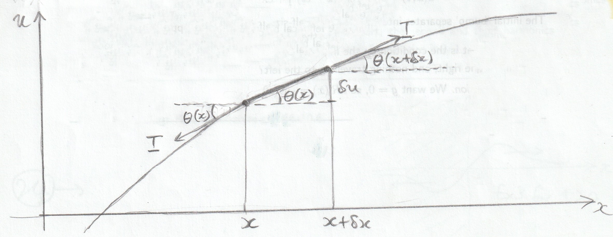
A thin string lies along the \(x\)-axis. It has density \(\rho\): the mass per unit length. Its tension (force) has constant magnitude \(T\), but its direction varies, since it points along the string. Let \(u(x,t)\) denote a small transverse displacement of the string, for example if it is plucked and then vibrates. Think of a small section of the string, from \(x\) to \(x+\delta x\), at an angle \(\theta\) to the horizontal. See Figure 2. The equation of motion is \[\rho\,\delta x\,\frac{\partial^2u}{\partial t^2}=T(\sin\theta)_{x+\delta x} -T(\sin\theta)_{x}\,.\] The displacement, and hence \(\theta\), are small, and so \(\sin\theta\approx\tan\theta=\delta u/\delta x\). Therefore our equation becomes \[\rho\,\frac{\partial^2u}{\partial t^2}=\frac{T}{\delta x} \left(\left[\frac{\delta u}{\delta x}\right]_{x+\delta x} -\left[\frac{\delta u}{\delta x}\right]_{x}\right).\] Now take the limit \(\delta x\to0\), and we get \[\frac{\partial^2u}{\partial t^2}=c^2\,\frac{\partial^2u}{\partial x^2},\] where \(c=\sqrt{T/\rho}\) is called the wave speed. This is the one-dimensional wave equation, and is an example of a partial differential equation.

Exercise. In a stringed instrument such as a guitar, the strings all have more-or-less the same length \(L\) and the same tension \(T\). The frequency (pitch) of the string is proportional to \(cL\), which has units of inverse time. The question is: if the pitch of string 1 is an octave higher (double the frequency) than that of string 2, what is the ratio \(\rho_2/\rho_1\) between the densities of the two strings?

Sketch of solution. \((c_1L)/(c_2L)=2\) gives \(\rho_2/\rho_1=4\).

8.2 d’Alembert’s solution.

It is very unusual to be able to solve a partial differential equation. But remarkably, one can write down the general solution of our one-dimensional wave equation. Let \(f(y)\) and \(g(z)\) be any two functions, and put \[u(x,t)=f(x-ct)+g(x+ct).\] It is easy to check, using the chain rule, that this is a solution of the wave equation. Clearly the first term describes a wave of shape \(f\) travelling to the right, while second term describes a wave of shape \(g\) travelling to the left. To see that we get all solutions this way, we must be able to satisfy arbitrary initial conditions. Namely, given two functions \(R(x)\) and \(S(x)\) describing the initial conditions \[u(x,0)=R(x), \quad \frac{\partial u}{\partial t}(x,0)=S(x)\] at time \(t=0\), we need to find \(f\) and \(g\) such that \(u(x,t)=f(x-ct)+g(x+ct)\) satisfies those conditions. The choice that does so is easily found: clearly \[R(x)=f(x)+g(x), \quad S(x)=-cf'(x)+cg'(x),\] and the second of these integrates to \[c^{-1}\int_0^x S(y)\,dy = -f(x)+g(x).\] Combining this with the \(R\)-equation then gives \(f\) and \(g\), in terms of \(R\) and \(\int S\). The result may be expressed as d’Alembert’s formula \[u(x,t)=\frac{1}{2}\left[R(x-ct)+R(x+ct)+ \frac{1}{c}\int_{x-ct}^{x+ct}S(y)\,dy\right].\]

Example 1. An infinite string is plucked (so \(S=0\)), with \(u(x,0)=\exp(-x^2)\). Then the d’Alembert formula gives \[u(x,t)=\tfrac{1}{2}\left\{\exp[-(x-ct)^2]+\exp[-(x+ct)^2]\right\}.\] The initial ‘bump’ separates into two identical half-size bumps travelling in opposite directions.

Exercise. What is the condition on the initial functions \(R(x)\) and \(S(x)\) which lead to a wave travelling to the right, and nothing travelling to the left?

Sketch of solution. We want \(g=0\), so \(cR'(x)=-S(x)\).

8.3 Examples and superposition.

Example 2. A string is struck (so \(R=0\)), with \(\partial u(x,0)/\partial t=2cx\exp(-x^2)\). Then the formula gives \[u(x,t)=\tfrac{1}{2}\left\{\exp[-(x-ct)^2]-\exp[-(x+ct)^2]\right\},\] representing two bumps of opposite sign, travelling in opposite directions.

Example 3. The displacement \(u(x,t)\) of a vibrating string satisfies the equation \(4u_{tt}=u_{xx}\), where the subscripts denote partial derivatives. Find the solution subject to the initial conditions \(u(x,0)=1/(1+x^2)\) and \(u_t(x,0)=x/(1+x^2)^2\). Solution: here \(c=1/2\) and \(c^{-1}\int S=-1/(1+x^2)\), giving \(u=1/[1+(x-t/2)^2]\).

Example 4. The string is attached to a wall at \(x=0\), and therefore obeys the boundary condition \(u(0,t)=0\) for all \(t\). What is the general solution? From \(u(x,t)=f(x-ct)+g(x+ct)\) we deduce that \(f(-ct)+g(ct)=0\) for all \(t\), and so the general solution is \[u(x,t)=f(x-ct)-f(-x-ct).\] Note that \(u(-x,t)=-u(x,t)\): the function \(u\) is odd in \(x\).

If we take \(f(y)=\exp(-y^2)\), then this looks like a ‘negative’ wave which comes in from the right, bounces off the wall, and then moves towards the right as a ‘positive’ wave. But we could also think of a ghost (image) wave inside the wall, which emerges to become the visible right-moving wave.

Superposition. Since the wave equation is linear, a sum of solutions is again a solution; this is called linear superposition. An example occurs with musical instruments (piano, guitar, flute etc) where the vibrating ‘thing’ is fixed at both ends. In that case, what you hear is a superposition of harmonics, the first harmonic being the fundamental frequency. Mathematically, the superposition is a Fourier series.

Exercise. Check that \(u_n(x,t)=\sin(nx)\sin(nct)\) is a solution of the wave equation, and that it satisfies the boundary conditions \(u_n(0,t)=0=u_n(\pi,t)\) for all integers \(n\). If your musical instrument produces a sound described by \[u(x,t)=\sum_{n=1}^{\infty} a_n u_n(x,t)\] where the \(a_n\) are constants, what is the ratio between the frequencies of the second (\(n=2\)) and the third (\(n=3\)) harmonic?

Sketch of solution. Checking is direct. For the last part, the second and third harmonics correspond to \(n=2\) and \(n=3\), and so the ratio of their frequencies is \(2/3\).

Further reading: Kibble-Berkshire section 10.6.

9.1 Rigid bodies and moment of inertia.

Suppose there are \(N\) masses \(m_1,m_2,\ldots,m_N\) at positions \({\bf r}_1,{\bf r}_2,\ldots,{\bf r}_N\). The centre of mass of this system is the point with position \[{\bf R}=\frac{m_1{\bf r}_1+m_2{\bf r}_2+\ldots+m_N{\bf r}_N}{m_1+m_2+\ldots+m_N}.\] Note that \(\dot{{\bf R}}=M^{-1}{\bf p}\), where \(M\) is the total mass and \({\bf p}\) is the total momentum. So if there are no net external forces acting, then \(\ddot{{\bf R}}={\bf 0}\) by conservation of total momentum. Then the centre of mass moves at constant velocity.

Rigid bodies. A rigid body is a collection of particles in which the distance between any two particles is fixed. Its motion is complicated, in general. If it is not rotating, then motion is simple: it behaves like a single particle located at its centre of mass. The next simplest case is rotation about a fixed axis \(P\), and we now restrict to this case. We have already met an example of such motion, namely the simple pendulum.

Moment of inertia. The moment of inertia of a particle of mass \(m\) about a line \(P\) is \(I=mr^2\), where \(r\) is the distance from the particle to the line. If there are several particles, we simply add: \[I = m_1r_1^2+m_2r_2^2+\ldots+m_Nr_N^2.\] For continuous systems, the sum becomes an integral.

Example 1. Four particles, each of mass \(m\), are attached to the corners of a light rigid square plate with sides of length \(L\). What is the moment of inertia \(I\) about an axis perpendicular to the square, passing through the centre of the square?

Solution. \(I=4m(L/\sqrt{2})^2=2mL^2\).

Exercise. For four particles of mass \(m\) at the corners of a square, as in Example 1, what is the moment of inertia \(I\) about an axis perpendicular to the square, passing through one of its corners?

Sketch of solution. \(I=0+2mL^2+m(L\sqrt{2})^2=4mL^2\).

9.2 Energy and dynamics.

Example 2. A uniform thin straight rod has length \(L\) and mass \(M\). It is free to rotate about an axis perpendicular to the rod, at one end of the rod. (This is an example of a compound pendulum, which means a rigid body that is free to rotate about a fixed horizontal axis under the influence of gravity.) What is its moment of inertia \(I\) about the specified axis?

Solution. The sum gets replaced by an integral. Think of a small length \(dx\) of the rod, at a distance \(x\) from the axis. It has moment of inertia \(dI=(M\,dx/L)x^2\), so \[I=\int_0^L (M\,dx/L)x^2 = \tfrac{1}{3}ML^2.\] The centre of mass is at \(x = M^{-1}\int_0^L (M\,dx/L)x = L/2\), in the middle as one would expect. Note that the moment of inertia depends on the position of the axis; for example, if the axis is at the centre of the rod, then \(I=ML^2/12\).

Kinetic energy. The position of a rigid body, rotating about a fixed axis, is specified by an angle \(\theta(t)\). Its angular velocity is \(\dot{\theta}\). The speed of a particle at distance \(r\) from the axis is \(v=r|\dot{\theta}|\), so its kinetic energy is \(\tfrac{1}{2}mv^2=\tfrac{1}{2}mr^2\dot{\theta}^2\). Adding (or integrating) over all the particles in the body then gives a kinetic energy \(K = I\dot{\theta}^2/2\), where \(I\) is the moment of inertia. Note the crucial feature that all the particles have the same \(\dot{\theta}\), since the body is rigid.

Total energy. If the external forces are conservative, one can define a potential energy \(V\) by summing or integrating over all the particles. Then the total energy \(E=K+V\) is conserved, and the equation \(dE/dt=0\) gives the equation of motion, namely \[I\ddot{\theta} = -V'(\theta).\]

Computing V. You can compute the potential energy \(V\) of a compound pendulum either by summing/integrating over all the particles, or by pretending that it is a simple pendulum with its total mass concentrated at the centre of mass. See Example 3.

Exercise. For the simple pendulum (notes 5.1), compute the moment of inertia \(I\) of the system about its pivot, and verify that the kinetic energy \(K\) is the same as before.

Sketch of solution. \(I=mL^2\) and so \(K=\tfrac{1}{2}mL^2\dot{\theta}^2\) as before.

9.3 Examples.

Example 3: compound pendulum. Take a uniform thin straight rod of length \(L\) and mass \(M\), as in Example 2. Its kinetic energy is \[K=\tfrac{1}{6}ML^2\dot{\theta}^2.\] Its potential energy is that of a particle of mass \(M\) located at the centre of mass, namely \[V(\theta) = \tfrac{1}{2}gML(1-\cos\theta).\] The total energy is \(E=K+V\), and the equation of motion is just \(dE/dt=0\), which gives \[\ddot{\theta}+\frac{3g}{2L}\sin\theta=0.\] This is the same as the equation of a simple pendulum of mass \(M\) and length \(2L/3\). So the period of small oscillations about the stable equilibrium is \(P=2\pi\sqrt{2L/(3g)}\).

Example 4. A uniform round pulley of mass \(M\) and radius \(L\) can rotate without friction about a fixed horizontal axis through its centre. A mass \(m\) is connected by a light string wound around the pulley, hanging downwards, with no slippage. Find the acceleration \(a\) of the mass.

Remark. Clearly we expect \(a\to0\) if \(m/M\to0\), and \(a\to g\) if \(M/m\to0\).

Solution. First compute the moment of inertia of the pulley about its axis. Easiest is to use polar coordinates \((r,\theta)\). Then \[I = \int\int M\left(\frac{r\,dr\,d\theta}{\pi L^2}\right)r^2 = \tfrac{1}{2}ML^2.\] The speed \(v\) of the mass is related to the angular speed by \(v=L\dot{\theta}\). Taking \(z\) to point downwards, the potential energy is \(V=-mgz\). Putting everything together gives the total energy \[E=\tfrac{1}{2}I\dot{\theta}^2 + \tfrac{1}{2}mv^2 - mgz =\tfrac{1}{2}(\tfrac{1}{2}M+m)\dot{z}^2-mgz.\] Using \(dE/dt=0\) and dividing by \(\dot{z}\) then leaves \[a=\ddot{z}=\frac{g}{1+M/(2m)}<g.\]

Exercise. For a compound pendulum made up of a rod of length \(L\) and mass \(M\) as in Example 2, plus a mass \(m\) at its end, compute the kinetic energy \(K\) and the potential energy \(V\).

Sketch of solution. Just add. So \(K=(\tfrac{1}{6}M+\tfrac{1}{2}m)L^2\dot{\theta}^2\) and \[V=gML(1-\tfrac{1}{2}\cos\theta)+gmL(1-\cos\theta).\]

Further reading: Kibble-Berkshire sections 8.1, 9.2; Gregory sections 2.4, 3.5, 9.3, 9.4, 11.1, 11.3, 11.6, Appendix.

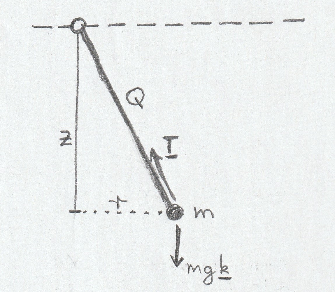
Problem. A mass \(m\) is attached to one end of a light rigid rod of length \(Q\), which is free to pivot at its other end, in any direction. Gravity acts downwards as usual. Initially the rod is horizontal, and its initial velocity \({\bf u}\) is also horizontal. In the subsequent motion, what depth \(D\) below the horizontal does the rod reach?

Note the trivial cases \(D=0\) if \(g=0\) (rotating horizontally), and \(D=Q\) if \(u=0\) (the simple pendulum, moving in a vertical plane). Let us take the origin \({\bf 0}\) to be at the pivot, the \(z\)-axis and \({\bf k}\) to be downwards, and polar coordinates \((r,\theta)\) horizontal. Let \({\bf R}=r{\bf e}_r+z{\bf k}\) denote the position of the mass. See Figure 3. Note that \[{\bf R}\cdot{\bf R}=z^2+r^2=Q^2 \quad\mbox{and}\quad \dot{{\bf R}}=\dot{r}{\bf e}_r+r\dot{\theta}{\bf e}_\theta+\dot{z}{\bf k}.\] The forces acting on the mass are gravity \(mg{\bf k}\), and a central force \({\bf T}\) (the tension along the rod, which keeps \({\bf R}\cdot{\bf R}=Q^2\)). Define \(E=\tfrac{1}{2}m \dot{{\bf R}}\cdot \dot{{\bf R}} -mgz\), namely the kinetic energy plus the gravitational potential energy (note the minus sign in the latter, because \(z\) increases downwards). Claim: \(E\) is conserved. Proof: note that \(\dot{z}={\bf k}\cdot \dot{{\bf R}}\). Thus \[\frac{dE}{dt}=m\dot{{\bf R}}\cdot\ddot{{\bf R}}-mg{\bf k}\cdot \dot{{\bf R}} =\dot{{\bf R}}\cdot(mg{\bf k}+{\bf T})-mg{\bf k}\cdot \dot{{\bf R}}=\dot{{\bf R}}\cdot{\bf T}.\] Now \({\bf R}\cdot{\bf R}=Q^2\) implies that \({\bf R}\cdot\dot{{\bf R}}=0\), so \(\dot{{\bf R}}\cdot{\bf T}=0\) since \({\bf T}\) is anti-parallel to \({\bf R}\). QED.

Next, angular momentum about \({\bf 0}\) is not conserved, since the gravitational force exerts torque about the pivot (note that \({\bf T}\), being a central force, does not exert torque). But gravity acts in a fixed direction, and so the component of angular momentum in that direction is conserved, as we now prove. Claim: \(L_z={\bf L}\cdot{\bf k}\) is conserved. Proof: \[\begin{aligned} \frac{d}{dt}{\bf L}\cdot{\bf k}&= m\frac{d}{dt}({\bf R}\times\dot{{\bf R}})\cdot{\bf k}\\ &=m{\bf R}\times\ddot{{\bf R}}\cdot{\bf k}\\ &={\bf R}\times(mg{\bf k}+{\bf T})\cdot{\bf k}\\ &=mg({\bf R}\times{\bf k}\cdot{\bf k})+({\bf R}\times{\bf T})\cdot{\bf k}\\ &=0+0=0. \quad {\rm QED.}\end{aligned}\]

Now in our case, we have \[\begin{aligned} L_z &= m(r{\bf e}_r+z{\bf k})\times(\dot{r}{\bf e}_r+r\dot{\theta}{\bf e}_\theta+\dot{z}{\bf k})\cdot{\bf k}\\ &= m(r{\bf e}_r)\times(r\dot{\theta}{\bf e}_\theta)\cdot{\bf k}\\ &=mr^2\dot{\theta},\end{aligned}\] and \(E=\tfrac{1}{2}m(\dot{r}^2+r^2\dot{\theta}^2+\dot{z}^2)-mgz\). The initial conditions give \(L_z=mQu\) and \(E=\tfrac{1}{2}mu^2\). So \[u^2=\dot{r}^2+r^2\dot{\theta}^2+\dot{z}^2-2gz =(z^2\dot{z}^2+Q^2u^2)/r^2+\dot{z}^2-2gz,\] using \(r\dot{r}+z\dot{z}=0\) which follows from \(z^2+r^2=Q^2\). Eliminating \(r\) altogether then gives \(Q^2\dot{z}^2=H(z)\) where \[H(z)=-2gz^3-u^2z^2+2gQ^2z.\] Now \(z\) is restricted by the condition \(H(z)\geq0\), giving \(0\leq z\leq D\) where \[D=\frac{1}{4g}\left(-u^2+\sqrt{u^4+16g^2Q^2}\right).\] So we see that the pendulum goes round in the \(\theta\)-direction, as well as oscillating vertically between \(z=0\) and \(z=D\). Exercise: show that \(D\leq Q\).