AMV II Epiphany Exercises 2023
Contents
1 Unit 1. Non Cartesian systems.
You are not asked to memorise the formulas giving the cylindrical polar and spherical polar coordinates in AMV II. In an exam paper, they would be given to you if necessary. It would be good if you could remember the change to polar coordinates in two dimensions though.
Polar coordinates: with , .
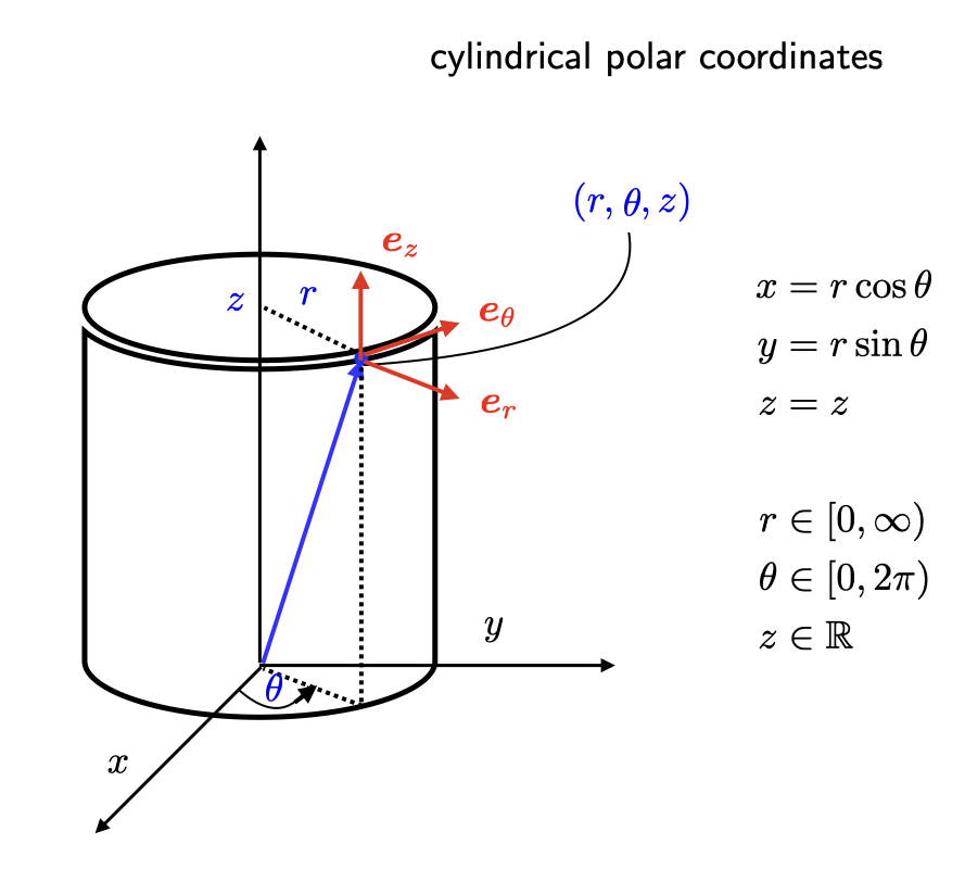
Cylindrical polar coordinates:
with , and .
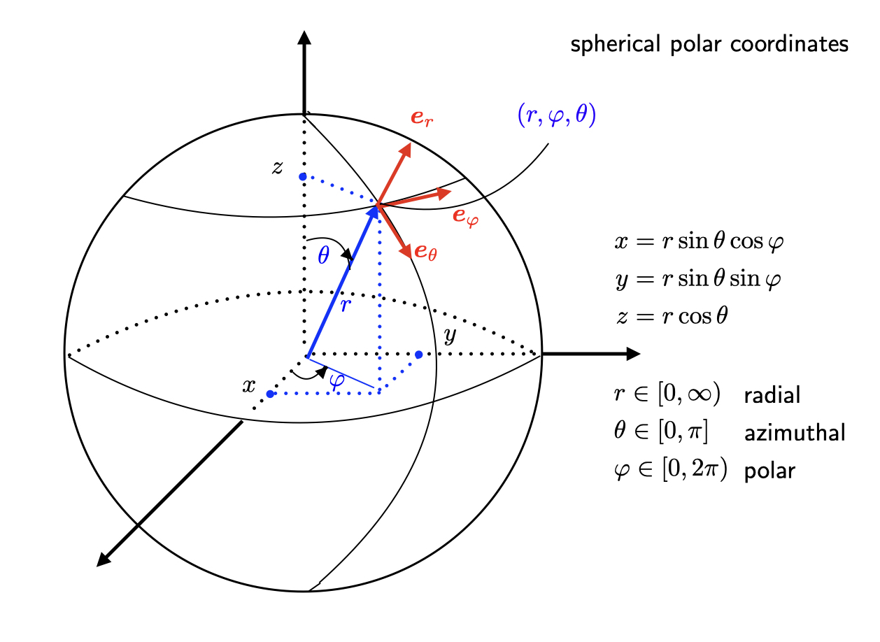
Spherical polar coordinates: with , , .
 |
 |
1.1 Double and triple integrals in orthogonal curvilinear coordinates
Exercise 1.1
The following equations are given in spherical polar coordinates. Interpret each of them geometrically.
Exercise 1.2
-
(a)
Find an equation in spherical polar coordinates for the sphere of equation
-
(b)
Express the upper-half of the ball by giving the relevant ranges of the three spherical polar coordinates .
Exercise 1.3 (TUT 1)
By expressing both the integrand and the surface element in spherical polar coordinates, evaluate the surface integral
where is an infinitesimal surface element on the surface of equation , .
Exercise 1.4
Use cylindrical polar coordinates to calculate
for the region .
Exercise 1.5 (Extension exercise)
Use cylindrical polar coordinates to find the volume of the solid bounded above by the plane and below by the paraboloid of equation .
1.2 Differential operators in curvilinear coordinates
The convention here is that form a right-handed basis in Cartesian coordinates, that is, .
Exercise 1.6
Express the differential equation
with a function of the coordinates in cylindrical polar coordinates.The variable is often labelling time in problems.
Exercise 1.7 (TUT 1)
Represent the vector in cylindrical polar coordinates and state what and are.
Exercise 1.8 (TUT 1)
Calculate for in spherical polar coordinates, with
You may use the formula
where and are the scale factors for spherical polar coordinates.
Exercise 1.9 (Extension exercise)
Let the Cartesian coordinates of any point in be expressed as functions of so that
and a positive constant. We shall call the system with coordinates the system.
-
(a)
Is the system orthogonal?
-
(b)
Calculate the scale factors and .
-
(c)
Give the unit vectors in the Cartesian basis.
-
(d)
Calculate the gradient in the basis of the system.
-
(e)
Express and in terms of and .
-
(f)
Given that
calculate the curl of the vector field (i.e. ) in the system.
-
(g)
Give the form of the Laplacian in this coordinate system.
Exercise 1.10 (GRAD 1)
-
(a)
Write the curve in polar coordinates. [2 marks]
-
(b)
Test this curve for symmetries (you may decide to work from the equation in Cartesian or polar coordinates for this). [2 marks]
-
(c)
Sketch the curve. [2 marks]
-
(d)
Evaluate the area of the region in the xy-plane bounded by the curve. [4 marks]
Exercise 1.11 (GRAD 1)
-
(a)
Calculate the Laplacian for the vector field in cylindrical polar coordinates. [5 marks]
-
(b)
Rework the same problem in Cartesian coordinates and show that the two results coincide (as they should). [5 marks]
2 Unit 2: Generalised functions
Exercise 2.1
Let be the unit step function defined on as
Give a definition and sketch the following functions,
-
(a)
for
-
(b)
for
-
(c)
-
(d)
(TUT 2)
-
(e)
Exercise 2.2
Given that, in the sense of distributions,
calculate, for ,
-
(a)
(TUT 2)
-
(b)
-
(c)
Exercise 2.3
By integrating both sides against an arbitrary test function , find the coefficients and , and possibly the constant in the following generalised identities,
-
(a)
(TUT 2) .
-
(b)
,
-
(c)
(TUT 2)
where denotes the second derivative of the Dirac delta distribution.
Exercise 2.4
By integrating both sides against an arbitrary test function , find the coefficients and in the following generalised identities,
-
(a)
-
(b)
.
-
(c)
, where is a real constant.
Exercise 2.5
By integrating both sides against an arbitrary test function find the coefficients and in the following generalised function identity,
where and are constants, with . Justify your steps fully.
Exercise 2.6
Give an expression for the charge density function of a ring of charge Q and radius centred at the origin and lying in the -plane
-
(a)
in cylindrical polar coordinates.
-
(b)
in spherical polar coordinates.
Then use spherical polar coordinates to calculate the electric potential resulting from that ring distribution of charge at a point on the -axis,
where is the vacuum permittivity constant and is the volume element expressed in the primed coordinates.
Exercise 2.7
-
(a)
(TUT 2) Show that the generalised function satisfies the generalised function relation for arbitrary constants. Justify your steps fully.
-
(b)
Learning from the shape of the solution to in part 1, what would you propose as the generalised solution to the relation ? and as the generalised solution to the relation for ? Give a very brief argument to support your answers.
Exercise 2.8
-
(a)
Let be a function with a unique zero at in an open interval . If this zero is simple (i.e. has multiplicity one) and if on the interval, then show that
(2.1) How is this relation modified if instead?
-
(b)
Use the relations obtained in part (a) to derive the equality
(2.2)
Exercise 2.9
-
(a)
Why can one consider the distribution as an antiderivative of the regular distribution , which is associated with the Heaviside (unit step) function?
-
(b)
Using induction, show that
(2.3)
Exercise 2.10
Consider the first order differential equation
What is its most general solution in the sense of distributions? Justify your answer fully by proving that your candidate solution satisfies the differential equation in the sense of distributions.
Exercise 2.11
Suppose you wish to solve the following ‘algebraic’ equation for the generalised function ,
| (2.4) |
where is a given smooth function. According to the sifting property of a factor of the delta function (see formula (2.12) in the lecture notes), if vanishes at some point , then the generalised function
satisfies (2.4). Knowing this, can you find the generalised solution of the following equations in terms of and its derivatives?
-
(a)
-
(b)
-
(c)
Exercise 2.12
Determine which of the following are piecewise continuous, piecewise
smooth or neither:
-
(a)
for , for .
-
(b)
for .
-
(c)
for and , .
-
(d)
for and , .
-
(e)
for and , .
Exercise 2.13 (GRAD 2)
Consider the function defined as
-
(a)
Is piecewise smooth? Justify fully. [3 marks]
-
(b)
Rewrite with the help of the unit step function defined as [3 marks]
-
(c)
Calculate the derivative of in the sense of distributions. [4 marks]
Exercise 2.14 (GRAD 2)
-
(a)
Consider the function and calculate, for any test function , the integral [4 marks]
where is the Dirac delta distribution.
-
(b)
Consider the distribution , where is the Dirac delta distribution dilated by a factor .
-
(i)
For which value of and do we have the following equalities of distributions? Justify your answers by integrating both sides against an arbitrary test function .
-
(1)
[2 marks]
-
(2)
[2 marks]
-
(1)
-
(ii)
Can you infer a basic identity satisfied by ‘in the sense of distributions’ from the results you obtained in part (i)(1) and part (i)(2)? [2 marks]
-
(i)
3 Unit 3: Sturm-Liouville Theory
Exercise 3.1
Show that the integral
defines an inner product on the quotient space , where is the set of all square-integrable functions that are non-zero on a set of Lebesgue measure zero, i.e. verify the axioms of a Hermitian inner product, justifying your claims.
Exercise 3.2
Show that the operator where is bounded.
We recall the definition of the space below (you should think of as being in this exercise). Definition: Let be the subspace of of all square-summable sequences, i.e. sequences of type , with a complex-valued function and
On that space, the inner product is given by
and the induced norm is given by .
Exercise 3.3
Convert the following linear second order differential operators into Sturm-Liouville form:
-
(a)
for .
-
(b)
for constant and .
-
(c)
for constant and
-
(d)
(TUT 3) for
-
(e)
for constant and
-
(f)
for constant and
Exercise 3.4
Consider the linear second order differential operator,
with non zero real constants.
-
(a)
Justify why is not formally self-adjoint.
-
(b)
Convert into Sturm-Liouville form.
Exercise 3.5
Consider the Sturm-Liouville operator with real-valued functions and .
-
(a)
(TUT 3) Which conditions would you put on at the boundaries of the interval to ensure that the Sturm-Liouville operator is not just formally self-adjoint, but such that the boundary terms in Green’s formula vanish irrespective of the boundary conditions one might put on the functions and acted upon by in a BVP problem?
-
(b)
Using your findings in part , determine the ‘natural’ interval over which each of the following Sturm-Liouville operator is self-adjoint. By ‘natural’, we mean ‘as determined by the boundary conditions on ’.
-
(i)
(TUT 3) with
-
(ii)
for .
-
(iii)
-
(i)
Exercise 3.6 (TUT 3)
Consider the boundary value problem (BVP) for ,
Suppose is a solution to this BVP and write it in the form What is the BVP satisfied by ? Is it self-adjoint?
Exercise 3.7
Consider the boundary value problem (BVP) for ,
Suppose is a solution to this BVP and write it in the form What is the BVP for ? Is it self-adjoint?
Exercise 3.8
Revisit exercises 3.6 and 3.7 above and compare the given initial BVP (for ) to the BVP (for ) that you have obtained in tutorials and in your formative assignment.
-
(a)
At the light of these two specific examples, and using the same notations for and , find the general form of the function for all that will ensure the BVP for has homogeneous Dirichlet boundary conditions. You may set the initial BVP on as
with a Sturm-Liouville operator and a source term. You may further assume that all functions are ‘sufficiently well-behaved’.
-
(b)
Is the BVP for self-adjoint? Justify.
Exercise 3.9
Consider the Sturm-Liouville operator acting on functions defined on the interval . Find adjoint boundary conditions in the following cases. (i) Neumann ; (ii) Periodic ; (iii) Initial . Which boundary conditions are self-adjoint? (for part (b), assume that is a nowhere vanishing periodic function on , i.e. ).
Exercise 3.10
Let
be a Sturm-Liouville operator with , and . Consider the BVP ( being a bounded function on ),
What are the conditions on the real constants for this BVP to be self-adjoint?
Exercise 3.11 (TUT 3)
Let be a smooth bounded region, and define an operator by
where are smooth functions on the closure of , which we denote . Show that
for all functions that vanish on the boundary of .
Exercise 3.12 (TUT 4)
Consider the regular Sturm-Liouville eigenvalue problem on
| (3.1) |
with where and are real-valued functions and on . Show that if for all , and if and , then all eigenvalues .
Exercise 3.13
Consider the Sturm-Liouville equation
with and two real-valued functions.
If and are two distinct solutions of the Sturm-Liouville equation, show that
is a constant.
Exercise 3.14 (GRAD 3)
Consider the Sturm-Liouville eigenvalue problem on for ,
Find the eigenvalues and the normalised eigenfunctions of the problem.
(Hint: In the course of solving this problem, you will encounter a differential equation of the Cauchy-Euler type, i.e. of the form
To solve it, set to obtain a differential equation with constant coefficients in the variable .)
Exercise 3.15
Consider the Sturm-Liouville eigenvalue problem on given by,
Find the eigenvalues and the normalised eigenfunctions (assume ).
Exercise 3.16
Consider the BVP on given by
-
(a)
Identify the Sturm-Liouville operator and the weight when the differential equation appearing in the BVP is rewritten as the eigenvalue equation .
-
(b)
Find the eigenvalues and the normalised eigenfunctions of the SL eigenvalue problem
Exercise 3.17 (GRAD 3)
-
(a)
Write the differential equation
in Sturm-Liouville form, i.e. identify the Sturm-Liouville operator , the weight and the parameter when is rewritten in the form .
-
(b)
What is the natural interval of definition for this Sturm-Liouville eigenvalue equation?
-
(c)
The eigenfunctions of this Sturm-Liouville problem associated with the eigenvalues are given by
Distinct eigenfunctions are mutually orthogonal w.r.t. the inner product . Check this statement for and . (You may use the result for )
Exercise 3.18
Consider the Sturm-Liouville eigenvalue problem on ,
Find the eigenvalues of this problem, and obtain the corresponding normalised eigenfunctions .
Exercise 3.19 (TUT 4)
Consider the following Sturm-Liouville problem on
-
(a)
Show that all the eigenvalues are positive.
-
(b)
Solve the problem.
Exercise 3.20
Use the method of eigenfunctions expansion to solve the inhomogeneous problem on given by
Exercise 3.21 (TUT 4)
Solve the following BVP problem on
using an eigenfunction expansion.
Exercise 3.22 (TUT 4)
Construct the generalised Fourier series expansion for the function
where the set is the set of orthonormal eigenfunctions stemming from a Sturm-Liouville eigenvalue problem on the interval with weight . Calculate and and compare with and .
4 Unit 4 Green’s functions
4.1 Green’s functions for ODEs
Exercise 4.1 (GRAD 4)
Solve the forced oscillator problem on using the ‘first shade of Green’:
All steps of the method used must be worked out in detail.
Exercise 4.2
The equation of motion for a driven damped harmonic oscillator can be written
with . If it starts from rest with and ,
-
(a)
find the corresponding Green’s function and verify that it can be written as a function of only.
-
(b)
find the explicit solution when the driving force is the unit step function, i.e.
Exercise 4.3 (TUT 5)
Consider the Green’s function defined on , ,
-
(a)
Show that the function defined by
satisfies the equation , where can be an arbitrary continuous function.
-
(b)
Show that for any , but that depends on the form of .
Exercise 4.4
Show that the Green’s function
is symmetric in the exchange of and whenever the BVP on is given by for a self-adjoint differential operator .
Exercise 4.5
Solve the following IN/HOM BVP on ,
by first calculating the relevant Green’s function.
Exercise 4.6
Find the Green’s function satisfying
Exercise 4.7 (TUT 5)
Solve the BVP
for using Green’s functions.
Exercise 4.8 (TUT 5)
Consider again the BVP on of the previous exercise, namely
Let and be two linearly independent solutions of the homogeneous differential equation associated with the given BVP, i.e. solutions of , with boundary conditions and .
Show that the function defined as
yields the Green’s function found in Exercise 4.7.
4.2 Green’s functions for PDEs
Exercise 4.9
Fix the point in the plane and check that the function
where is the distance between and is a solution to the problem
except at .
Exercise 4.10
Method of images
-
1.
Construct the Green’s function for the Dirichlet Poisson problem
where the wedge domain has boundary .
-
2.
Show by a direct calculation using what you found for that , where , with the fundamental solution to Laplace’s equation in two dimensions.
-
3.
Check that on the boundary, .
Exercise 4.11
Method of images
A line charge in the -direction, of charge density , is placed at some position in the quarter space . Calculate the force per unit length on the line charge due to the presence of thin earthed plates along and .
Hint: The force per unit length on the line charge with charge density at position due to charges in the neighbourhood is , where the potential is the solution to Poisson’s equation (with constant)
| (4.1) |
in the quarter plane , with Dirichlet boundary conditions . To solve this problem, proceed in four steps
-
1.
Construct the Green’s function by the method of images, with the fundamental solution taken to be (see lecture notes). Draw a picture to help your reasoning.
-
2.
Check that the Green’s function you found is zero on the boundary and when
-
3.
Express the potential satisfying (4.1) in terms of the Green’s function
-
4.
Calculate the force experienced by the line charge at due to the presence of the image line charges of charge density .
Exercise 4.12
Method of images
Find the Green’s function for the Poisson Dirichlet problem on , with when and 0 otherwise.
Exercise 4.13 (extension)
Find the Poisson kernel for the Poisson Dirichlet problem of the previous question.