Project III: Statistics for spatial data
Jonathan Cumming
Spatial data can arise in many scientific and other contexts, including the environment, public health, agriculture, and geology. For example, we may gather air quality measurements at several monitoring stations to model and predict air pollution; or assess the average income in each UK postcode area as an indicator of deprivation; or observe the locations at which cases of a particular disease were observed to understand patterns of incidence and infection. The structure of these data sets and how we may model them varies greatly, but each clearly has an aspect that varies with the location. In the first of the examples, we control the locations and measure the data values; in the second, we have pre-defined regions and make a measurement for each area; and in the final example, we simply observe the locations where the disease is observed.
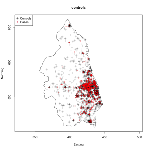
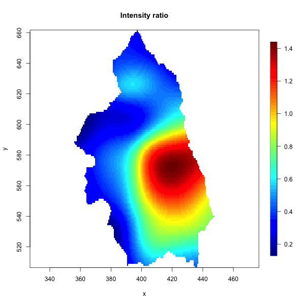
FIGURE 21.3: Cases of primary biliary cirrhosis and controls representing at-risk population (left) and intensity ratio (right) in north-eastern England between 1987 and 1994.
In all our examples, we can think of our data as corresponding to measurements of some quantity of interest, \(Y\), which varies as a function of its spatial location, \(s\). In the air quality example, we measure a real-valued Y at various continuous locations \(s\), and our goal is usually to predict the values of \(Y\) at unobserved locations. This is often called geostatistics and models hinge on the reasonable assumptions that \(Y\) will change smoothly and that nearby locations will likely have similar values of \(Y\), but more distant locations are less related. Interpolation methods, such as Gaussian processes or kriging are commonly used. The second example concerns areal data and has a similar setup but a far simpler structure to the locations \(s\).
Conversely, in the disease incidence example, \(Y\) is \(1\) at a particular location s if a case of the disease was observed there. This leads to point patterns and point processes, where we are interested in understanding the underlying spatial process that generates the pattern of points we observed. Then, given that process, we’re interested assessing whether, for example, the spatial process has a uniform rate everywhere, or whether there are clusters or hot spots indicating areas of higher risk - such as in the figure above.
After developing an understanding of the basic concepts and fundamental statistical models for spatial data, you may then take the project in whatever direction you find most interesting, which might include going deeper into study of particular methods, or focussing on analysis of a real-world data set.
This project has a focus on statistical methodology and data analysis. Familiarity with the statistical package R (or equivalent languages such as Python), general statistical concepts, and data analysis are essential.
Essential prior knowledge
- Statistical Inference II - for familiarity with standard statistical ideas and experience with R.
- (optional) Statistical Modelling II - helpful for understanding simple statistical models, but not essential
Further reading
This is a widely covered topic and many books contain suitable introductory material.
- Cressie N, Statistics for Spatial Data, 1991
- Moraga P, Spatial Statistics for Data Science: Theory and Practice with R, 2024.
- Schabenberger O, Gotway CA, Statistical methods for spatial data analysis, 2005.
- Ripley BD, Spatial Statistics, 1981.
- Waller LA, Gotway CA, Applied spatial statistics for public health data, 2004.
- Diggle P, Statistical analysis of spatial point patterns, 2003.